在线阅读地址:https://junhuatechlog.github.io/Play-with-ML-in-Python/
Jupyter notebook修改默认工作路径
在powershell下用jupyter notebook --generate-config生成配置文件: .jupyter/jupyter_notebook_config.py Jupyter notebook 使用安装路径作为默认路径,如果要修改默认路径,需要修改.jupyter/jupyter_notebook_config.py里的 c.ServerApp.root_dir 设置这个路径时,为了避免将字符串里路径的反斜杠解释为转义字符,有2种方法:
- 在反斜杠前面另加一个反斜杠,将其转义
- 使用原始字符串(raw string)的特性 - 在字符串前面加r. c.ServerApp.root_dir = r'C:\N-20KEPC0Y7KFA-Data\junhuawa\Documents\Play-with-ML-in-Python\src\04-kNN'
import sys sys.path.append('C:\Users\junhuawa\PycharmProjects\playML')
打开其他文件夹下的jpynb文件
在powershell prompt下,输入给jupyter notebook输入对应的目录
jupyter notebook C:\N-20KEPC0Y7KFA-Data\junhuawa\Documents\Play-with-ML-in-Python\src\Basics
python interpretor path
C:\Users\junhuawa\AppData\Local\anaconda3\python.exe
Settings/Project/Python Interpreter
Matplotlib
mdbook 创建和部署steps
根据 mdbook guide 在本地创建一个mdbook的repo.
mdbook init my-first-book
cd my-first-book
mdbook serve --open
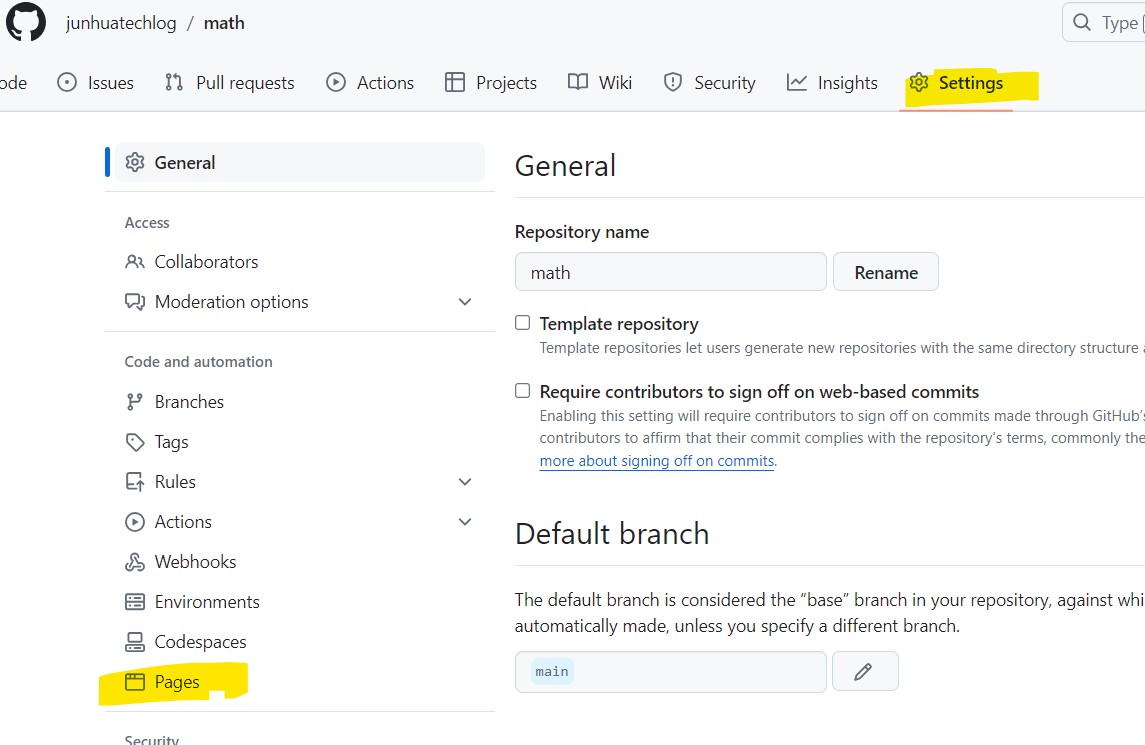
把 repo push 到 github server之后,需要设置 github pages,并设置 workflow (使用默认的 yml 文件就可以),使每一次commit都会trigger rebuild 和 redeployment. redeployment之后可以看到生成的book的link.


Numpy
Python class
类函数的第一个参数通常被称为self, 这个参数只会出现在类的定义中
from math import gcd
class Frac:
    """ Fractional class. A Frac is a pair of integers num, den(with den!=0) whose gcd is 1."""

    def __init__(self, n, d):# 类的构造函数
        """ Construct a Frac from integers n and d.
            Need error message if d =0!"""
        assert d != 0, "The denumeritor should not be 0!"
        hcf = gcd(n, d)
        self.num, self.den = n/hcf, d/hcf

    def __str__(self):
        """ Generate a string representation of a Frac. """
        if self.den == 1:
            return "%d" % (self.num)
        else:
            return "%d/%d" % (self.num, self.den)

    def __mul__(self, another):
        """ Multiply 2 Fracs to produce a Frac. """
        return self.num*another.num / (self.den*another.den)

    def __add__(self, another):
        """ Add 2 Fracs to produce a Frac. """
        return Frac(int(self.num*another.den+self.den*another.num), int(self.den*another.den))

    def __div__(self, another):
        """ Divide a Fracs to produce a new Frac. """
        return Frac(int(self.num*another.den), int(self.den*another.num))

    def __sub__(self, another):
        """ Sub a Fracs to produce a new Frac. """
        return Frac(int(self.num*another.den-self.den*another.num), int(self.den*another.den))
    def to_real(self):
        """ Return floating point value of Frac. """
        return float(self.num/float(self.den))

if __name__ == "__main__":
        a = Frac(3,7)
        b = Frac(24, 56)
        print("a.num = ",  a.num)
        print(", a.den =  ", a.den)
        print(a)
        print(b)
        print("floating point value of a is ", a.to_real())
        print("product = ", a*b)
        print("Sum = ", a+b)
        print("Sub = ", a - b)
        print(Frac(24, 1))
        print("Div = ", a.__div__(b))
        print("Div = ", a.__div__(b))
        #Frac(24, 0)
kNN - k Nearest Neighbors k近邻算法
欧拉距离
$$\sqrt{(x^{(a)} - x^{(b)})^2 + (y^{(a)} - y^{(b)})^2}$$
$$\sqrt{(x_1^{(a)} - x_1^{(b)})^2 + (x_2^{(a)} - x_2^{(b)})^2 + ... + (X_n^{(a)} - x_n^{(b)})^2}$$
$$\sqrt {\sum_{i=1}^n (X_i^{(a)} - X_i^{(b)})^2}$$
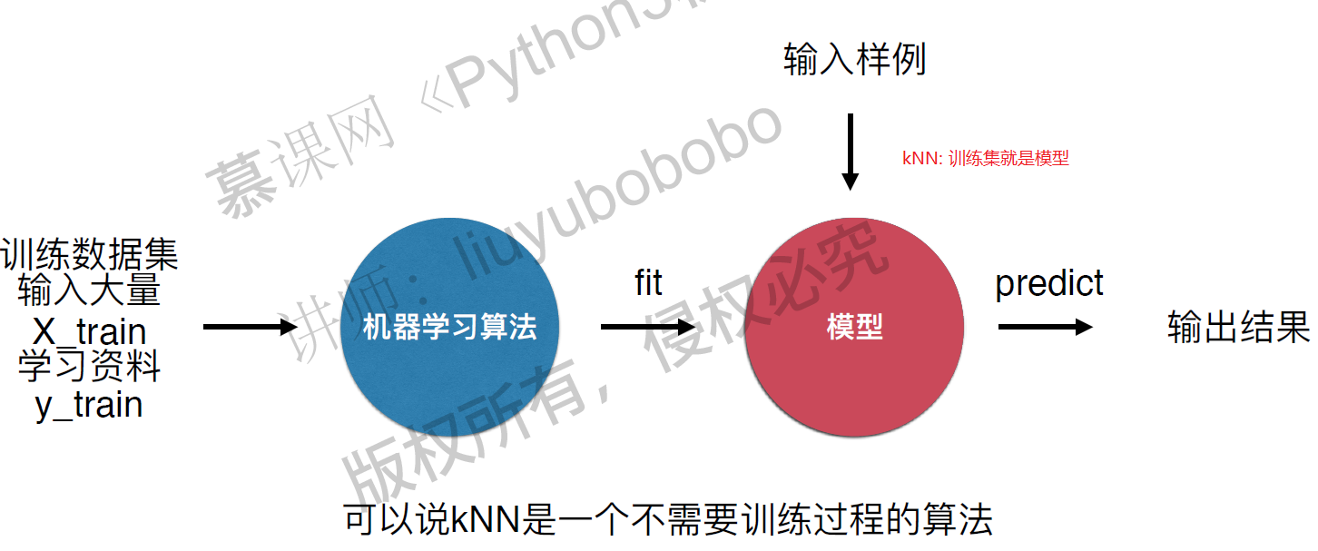 kNN算法是非常特殊的,可以被认为是没有模型的算法,为了和其他算法统一,可以认为训练数据集就是模型本身。
判断机器学习算法的性能
需要将数据集分成训练/测试数据集,通过测试数据直接判断模型的好坏!在模型进入真实环境前改进模型。 train test split
分类准确度 - accuracy
预测结果和样本结果一致的样本数占所有样本数的比例。
超参数和模型参数
超参数: 在机器学习算法运行前需要决定的参数, 比如k
模型参数: 算法在训练过程中学习到的参数
kNN算法没有模型参数,kNN算法中的k是典型的超参数。 寻找好的超参数依赖 - 领域知识(视觉搜索,自然语言处理) - 经验数值(kNN算法中k默认为5) - 实验搜索。
kNN算法中另一个超参数: 距离
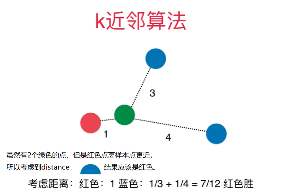 为了让kNN预测结果更合理,需要考虑距离的权重,通常用距离的倒数作为权重。
距离还可以解决平票的问题: 比如和样本点相连的3个点是3中类别,如果不考虑距离权重,则只能从3个中随机选一个作为预测结果,不合理.
为了让kNN预测结果更合理,需要考虑距离的权重,通常用距离的倒数作为权重。
距离还可以解决平票的问题: 比如和样本点相连的3个点是3中类别,如果不考虑距离权重,则只能从3个中随机选一个作为预测结果,不合理.
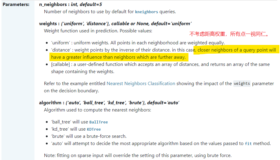
weights: - uniform - distance
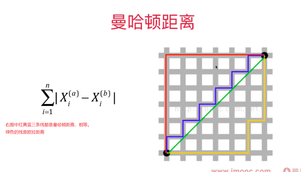
距离有:
- 欧拉距离 $\sqrt {\sum_{i=1}^n (X_i^{(a)} - X_i^{(b)})^2}$
- 曼哈顿距离 $\sum_{i=1}^n \left| X_i^{(a)} - X_i^{(b)} \right| $
代表两个样本点在每个维度上的距离的和
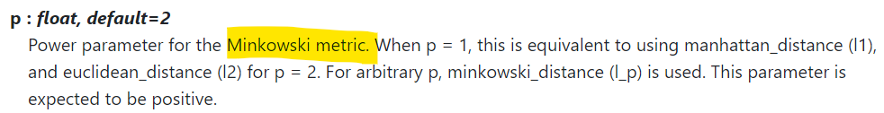
-  - 明可夫斯基距离 Minkowski Distance $(\sum_{i=1}^n {\left| X_i^{(a)} - X_i^{(b)} \right|}^p)^{\frac 1 p} $
更多距离定义, 可以用相似度来定义样本间的距离:
- 向量空间余弦相似度 Cosine Similarity
- 调整余弦相似度 Adjusted Cosine Similarity
- 皮尔森相关系数 Pearson Correlation Coefficient
- Jaccard 相似系数 Jaccard Coefficient
寻找超参数要用网格搜索:
import numpy as np
import matplotlib
import matplotlib.pyplot as plt
from sklearn import datasets
from sklearn.neighbors import KNeighborsClassifier
from sklearn.model_selection import GridSearchCV
from sklearn.model_selection import train_test_split

digits = datasets.load_digits()
X_train, X_test, y_train, y_test = train_test_split(digits.data, digits.target, test_size=0.2, random_state=600)

param_grid = [
    {
        'weights': ['uniform'],
        'n_neighbors': [i for i in range(1, 11)]
    },
    {
        'weights': ['distance'],
        'n_neighbors': [i for i in range(1, 11)],
        'p': [p for p in range(1, 6)]
    }
]

knn_clf = KNeighborsClassifier()
grid_search = GridSearchCV(knn_clf, param_grid, n_jobs = -1, verbose = 2)
grid_search.fit(X_train, y_train)

# 根据用户传入参数计算得到的参数
grid_search.best_estimator_
grid_search.best_score_
grid_search.best_params_
knn_clf = grid_search.best_estimator_
knn_clf.score(X_test, y_test)
Fitting 5 folds for each of 60 candidates, totalling 300 fits
KNeighborsClassifier(n_neighbors=1, p=3, weights='distance')
0.990251161440186
{'n_neighbors': 1, 'p': 3, 'weights': 'distance'}
0.9805555555555555
提升计算性能: n_jobs = -1, 用所有的核来计算
verbose: 整数值越大,输出的信息越多
GridSearchCV(knn_clf, param_grid, n_jobs = -1, verbose = 2)
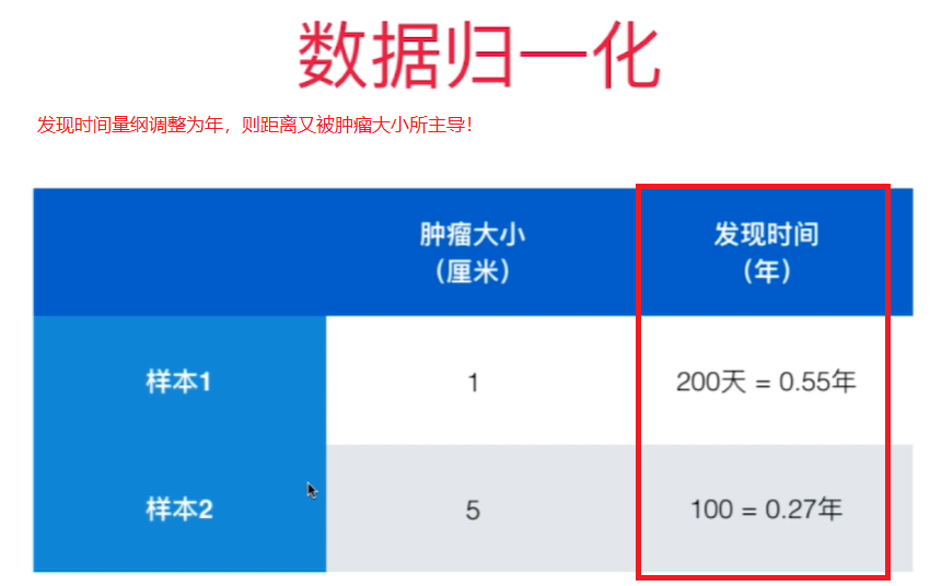
数据归一化 Feature Scaling
如果不做数据归一化,因为各个特征量纲不同, 某些特征的数值大小差距比其他特征的数值差距大很多,样本间的距离被个别数值差距大的特征主导。
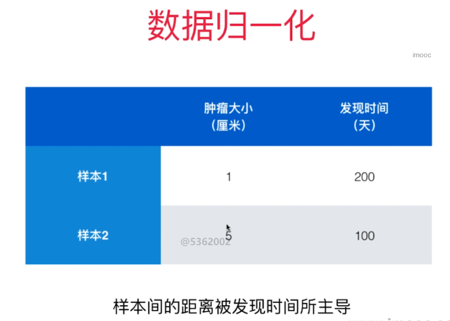
解决方案:将所有的数据映射到同一个尺度
-
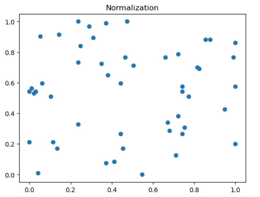
最值归一化: 把所有的值映射到0-1之间 - Normalization - 最简单的映射 $$x_{scale} = \frac {x - x_{min}} {x_{max} - x_{min}}$$
适用于数据分布有明显边界的地方, 比如学生的成绩,像素, 它受Outlier影响较大
不适合没有明显边界的情况,比如收入分布,有人收入很高,大部分人收入一般,映射后大部分人的值会很低。
-
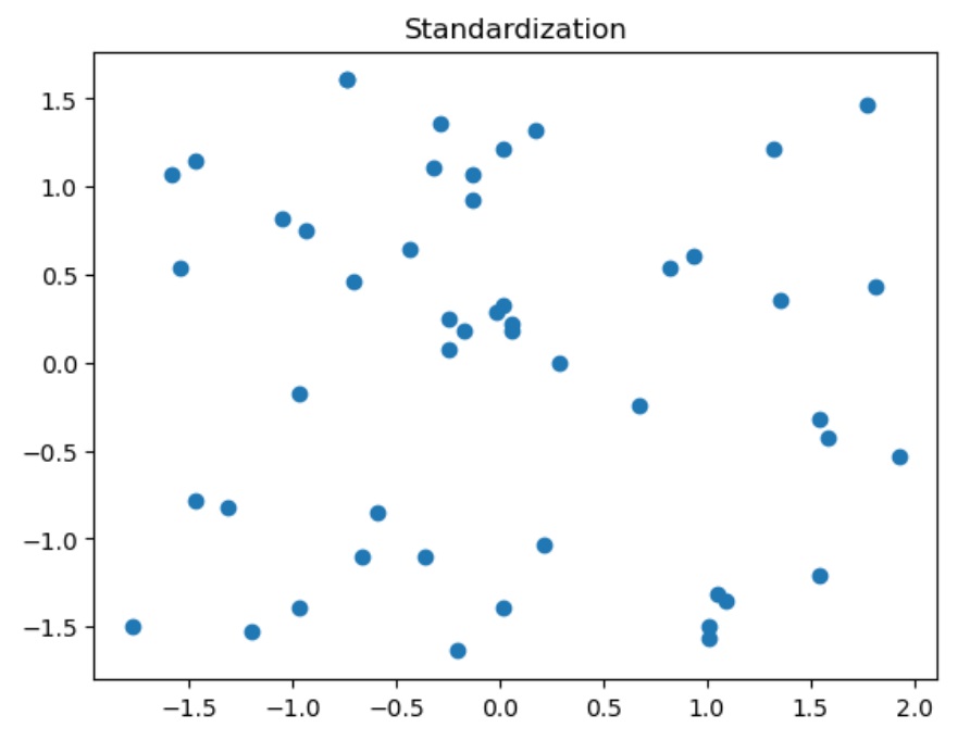
均值方差归一化- Standardization 把所有数据归一到均值为0, 方差为1的分布中。这样做了之后不能保证所有的值都在0-1之间,但保证均值为0, 方差为1, 也就不会形成有偏的数据。
适用于数据没有边界, 有可能存在极值(Outlier)的数据
如果数据有明显边界,用这个方法效果也是很好的。
所以,一般情况下,都用均值方差归一化
-
$$x_{scale} = \frac {x - x_{mean}} S$$ S为方差
import numpy as np
import matplotlib.pyplot as plt
X = np.random.randint(0, 100, (50, 2))
X = np.array(X, dtype='float')
#最值归一化
for i in range(0, 2):
    X[:,i] = (X[:, i] - np.min(X[:, i]))/(np.max(X[:, i]) - np.min(X[:, i]))
X[:, 0].mean(), X[:, 0].std()

plt.scatter(X[:, 0], X[:, 1])
plt.title("Normalization")
结果:均值不为0, 方差不为1
0.47422680412371127, 0.3155110806332136
# 均值方差归一化
for i in range(0, 2):
    X[:, i] = (X[:, i] - np.mean(X[:, i]))/np.std(X[:, i])
np.mean(X[:, 0]), np.std(X[:, 0]), np.mean(X[:, 1]), np.std(X[:, 1])

plt.scatter(X[:, 0], X[:, 1])
plt.title("Standardization")
结果:均值为0, 方差为1, 无偏数据
1.2878587085651815e-16, 1.0, 1.021405182655144e-16, 0.9999999999999999
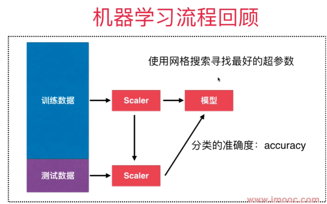
scikit-learn中的Scaler
均值方差归一化时,对训练数据集做归一化,测试数据集要用训练数据集的均值和方差做归一化。$\frac {x_{test} - mean_{train}} {{Std}_{train}}$
真实环境中很有可能无法得到所有测试数据的均值和方差。 对数据的归一化也是算法的一部分。
在sklearn中,需要保存训练数据的均值和方差,用于测试集用,所以封装了一个Scaler类, 在sklearn.preprocessing模块里。
- mean_
- std_
import numpy as np
import matplotlib.pyplot as plt
from sklearn import datasets
iris = datasets.load_iris()
X = iris.data
y = iris.target
from sklearn.model_selection import train_test_split
X_train, X_test, y_train, y_test = train_test_split(X, y, random_state=666)
from sklearn.preprocessing import StandardScaler
standardScaler = StandardScaler()
standardScaler.fit(X_train)
standardScaler.mean_
standardScaler.scale_ #描述数据分布范围,和std_一样,只是std_这个变量名在sklearn中弃用了。
结果:
array([5.825     , 3.09285714, 3.68571429, 1.16428571])
array([0.80239597, 0.4493476 , 1.75828941, 0.75543946])
数据归一化后做knn分类的效果:
X_train_standard = standardScaler.transform(X_train)
X_test_standard = standardScaler.transform(X_test)
from sklearn.neighbors import KNeighborsClassifier
knn_clf = KNeighborsClassifier(n_neighbors=3)
knn_clf.fit(X_train_standard, y_train)
knn_clf.score(X_test_standard, y_test)
knn_clf.score(X_test, y_test)
结果:
0.9736842105263158
0.34210526315789475 # 一定要用归一化后的测试数据做预测
更多思考
kNN算法天然的可以解决多分类问题,思想简单,效果强大。
也可以解决回归问题, 找到离样本点最近的k个节点, 求这几个点的平均值就是要求的点的值。 也可以用加权平均方法。
KNeighborsRegressor
缺点:
- 效率低下, m个样本,n个特征的情况下,每预测一个数据,需要O(m*n)的计算量 可以使用KD-Tree, ball-tree更快的求出k近邻。
- 高度数据相关, 对outlier更敏感。 比如k=3,在样本点附近有2个错误的值的点,则结果肯定出错。
- 预测结果不具有可解释性
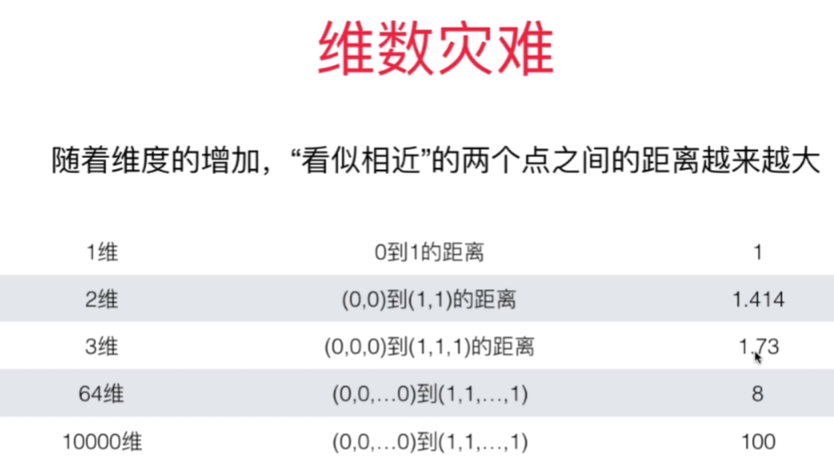
- 维数灾难 - 随着维度的增加,看似相近的两个点之间的距离越来越大。- 解决方法: 降维 PCA
线性回归 - Linear Regression
- 解决回归问题
- 是许多强大的非线性模型的基础
- 结果具有良好的可解释性
- 蕴含机器学习中的很多重要的思想
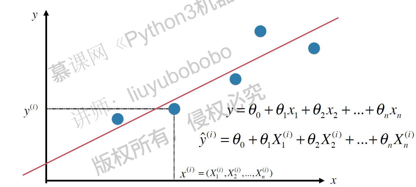
寻找一条直线,最大程度的“拟合”样本特征和样本输出标记之间的关系。
简单线性回归: 样本特征只有一个
目标函数: 使 $\sum_{i=1}^m (y^{(i)} - {\hat y}^{(i)})^2 $ 尽可能小. $$ {\hat y}^{(i)} = ax^{(i)} + b $$
即: 找到a和b,使得 $\sum_{i=1}^m (y^{(i)} - ax^{(i)} - b)^2 $ 尽可能小。

通过分析问题,确定问题的损失函数或者效用函数; 通过最优化损失函数或者效用函数,获得机器学习的模型。近乎所有的参数学习算法都是这样的套路。
最小二乘法解决简单线性回归问题: $$ a = \frac {\sum_{i=1}^m (x^{(i)} - \bar x)(y^{(i)} - \bar y)} {\sum_{i=1}^m (x^{i} - \bar x)^2}$$
$$ b = \bar y - a \bar x$$
回归算法的衡量 MSE vs. MAE
均方误差 MSE( Mean Squared Error ) - 量纲是平方
$$ \frac 1 m \sum_{i=1}^m (y_{test}^{(i)} - \hat y_{test}^{(i)})^2$$
均方根误差 RMSE(Root Mean Squared Error)
$$\sqrt {\frac 1 m \sum_{i=1}^m (y_{test}^{(i)} - \hat y_{test}^{(i)})^2} $$
平均绝对误差 MAE (Mean Absolute Error)
$$ \frac 1 m \sum_{i=1}^m \left| y_{test}^{(i)} - \hat y_{test}^{(i)} \right| $$
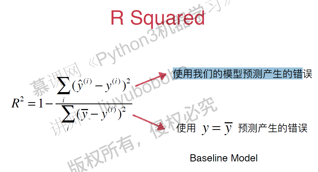
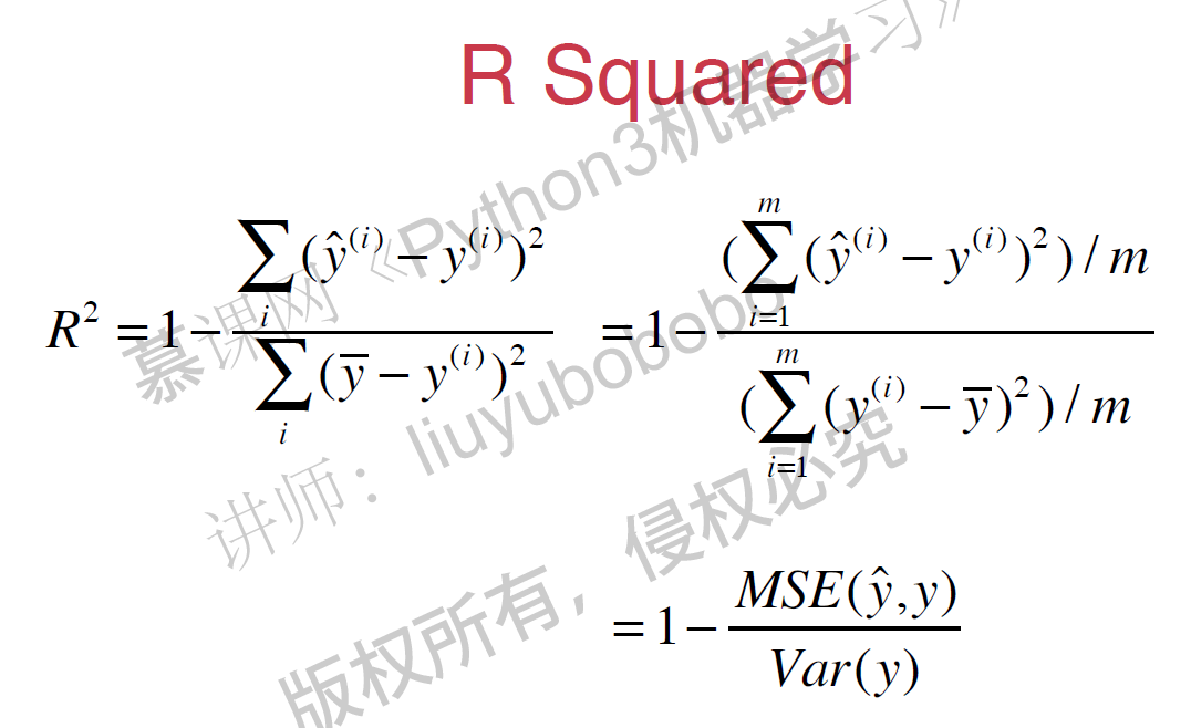
R Squared
$$R^2 = 1 - \frac {{SS}{residual}} {{SS}{total}}$$ $\frac {Resisual\ Sum\ of\ Squared} {Total\ Sum\ of\ Squares} $
$$R^2 = 1 - \frac {\sum_i (\hat y^{(i)} - y^{(i)})^2} {\sum_i (\bar y - y^{(i)})^2}$$
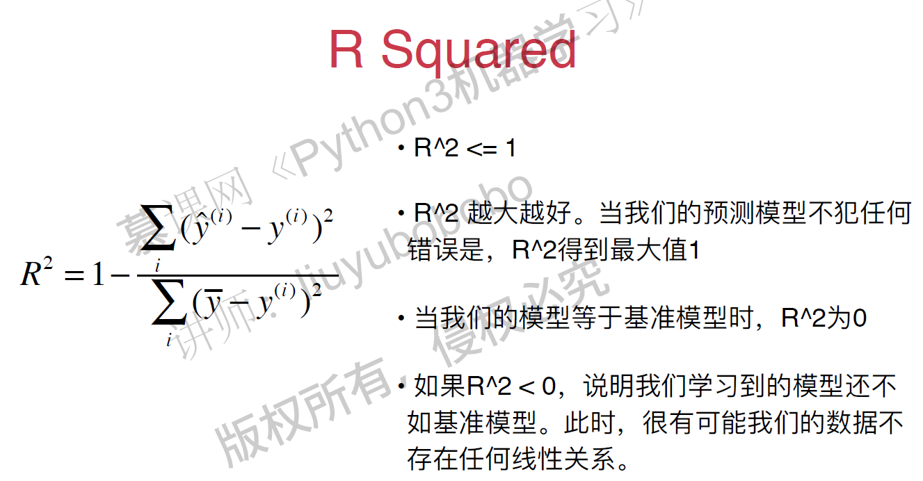
Scikit-Learn中的线性回归法,score默认为R Squared的值。
线性回归 - Linear Regression
- 解决回归问题
- 是许多强大的非线性模型的基础
- 结果具有良好的可解释性
- 蕴含机器学习中的很多重要的思想
寻找一条直线,最大程度的“拟合”样本特征和样本输出标记之间的关系。
简单线性回归: 样本特征只有一个
目标函数: 使 $\sum_{i=1}^m (y^{(i)} - {\hat y}^{(i)})^2 $ 尽可能小. $$ {\hat y}^{(i)} = ax^{(i)} + b $$
即: 找到a和b,使得 $\sum_{i=1}^m (y^{(i)} - ax^{(i)} - b)^2 $ 尽可能小。
通过分析问题,确定问题的损失函数或者效用函数; 通过最优化损失函数或者效用函数,获得机器学习的模型。近乎所有的参数学习算法都是这样的套路。
最小二乘法解决简单线性回归问题: $$ a = \frac {\sum_{i=1}^m (x^{(i)} - \bar x)(y^{(i)} - \bar y)} {\sum_{i=1}^m (x^{i} - \bar x)^2}$$
$$ b = \bar y - a \bar x$$
回归算法的衡量 MSE vs. MAE
均方误差 MSE( Mean Squared Error ) - 量纲是平方
$$ \frac 1 m \sum_{i=1}^m (y_{test}^{(i)} - \hat y_{test}^{(i)})^2$$
均方根误差 RMSE(Root Mean Squared Error)
$$\sqrt {\frac 1 m \sum_{i=1}^m (y_{test}^{(i)} - \hat y_{test}^{(i)})^2} $$
平均绝对误差 MAE (Mean Absolute Error)
$$ \frac 1 m \sum_{i=1}^m \left| y_{test}^{(i)} - \hat y_{test}^{(i)} \right| $$
R Squared
$$R^2 = 1 - \frac {{SS}{residual}} {{SS}{total}}$$ $\frac {Resisual\ Sum\ of\ Squared} {Total\ Sum\ of\ Squares} $
$$R^2 = 1 - \frac {\sum_i (\hat y^{(i)} - y^{(i)})^2} {\sum_i (\bar y - y^{(i)})^2}$$
Scikit-Learn中的线性回归法,score默认为R Squared的值。
多元线性回归
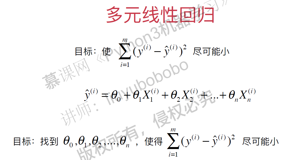
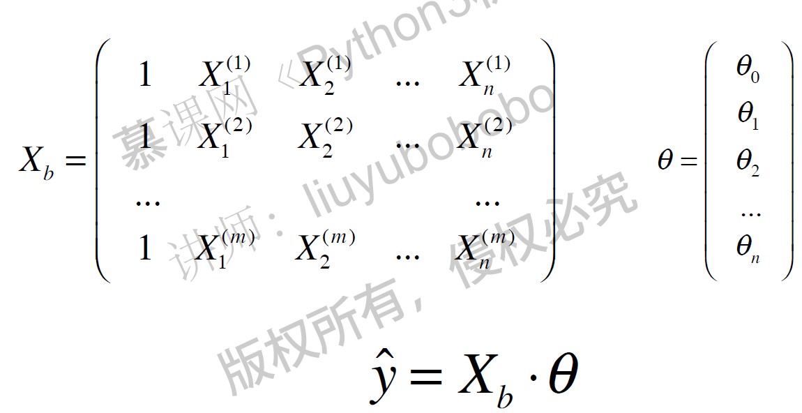
多元线性回归的目标函数: $$\hat y = X_b \cdot \theta $$ 使$ \sum_{i=1}^m(y^{(i)} - {\hat y}^{(i)})^2 $ 尽可能小。 即使 $ (y - X_b \cdot \theta)^T (y-X_b \cdot \theta)$ 尽可能小。
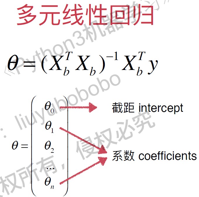
以下是多元线性回归的正规方程解( Normal Equation), 时间复杂度高: $O(n^3)$ (优化后是 $O(n^{2.4})$), 优点是不需要对数据做归一化处理。
$$ \theta = (X_b^TX_b)^{-1} X_b^T y $$
总结:
| kNN | Linear Regression |
|---|---|
| 非参数学习 | 典型的参数学习算法 |
| 既可以解决分类问题,又可以解决回归问题 | 虽然是很多分类算法的基础(Logistic Regression), 但是只能解决回归问题 |
| 对数据没有假设 | 对数据有线性的假设 |
| 对数据无解释性 | 对数据有强解释性 |
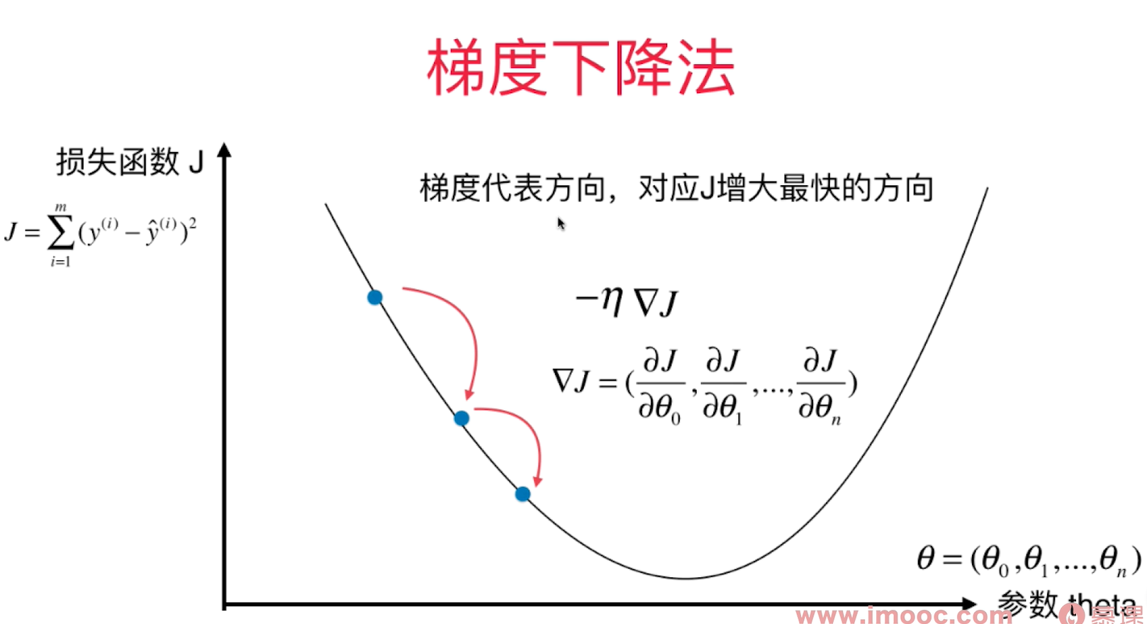
梯度下降法 - Gradient Descent
不是一个机器学习算法,不能解决分类,回归问题;
是一种基于搜索的最优化方法 - 最优化一个损失函数(loss function) - 在机器学习领域最小化损失函数的最为常用的一种方法
最大化一个效用函数则用梯度上升法
很多模型得不到最优数学解,所以只能通过搜索策略找到最优解。
寻找一个参数 $\theta$, 使得损失函数J取得最小值!
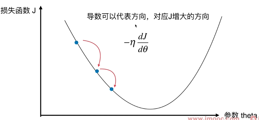
直线方程中,导数代表斜率, 在曲线方程中,导数代表切线斜率
导数代表 $\theta$单位变化时,损失函数J相应的变化。
导数可以代表方向,对应J增大的方向。
导数为负值,则表示theta减小时,J增大;我们要想往J减小的方向前进,则 $\theta+一个导数*(-\eta)$。
对多维函数来说,导数就是对应的梯度。
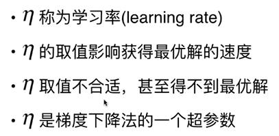
$\eta$ - 步长
把目标函数J当作一个山谷,一个球会自然的滚落下来,梯度下降法就好像在模拟这个球的滚落过程。 当球滚落到谷底时,相应的找到了J的最小值。滚落的速度由$ \eta $决定。
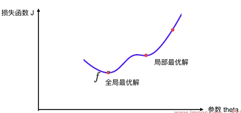
并不是所有的函数都有唯一的极值点, 上图有2个极小值(导数=0),这个极小值有可能只是局部最优解,而不是全局最优解 - 搜索过程中会遇到的问题
解决方案:
多次运行, 随机化初始点 - 初始点也是一个超参数
线性回归法的损失函数具有唯一的最优解。
梯度下降法的超参数:
- eta - 步长
- 初始点
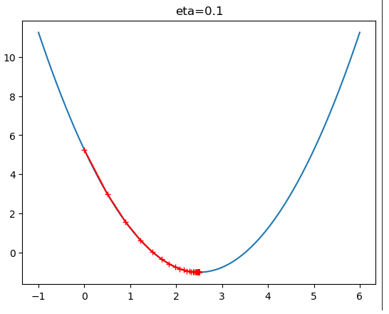
模拟实现梯度下降法
import numpy as np
import matplotlib.pyplot as plt
plot_x = np.linspace(-1, 6, 141)

def dJ(theta):#求theta点对应的梯度
    return 2*(theta - 2.5)

def J(theta):#损耗函数
    try:
        return (theta-2.5)**2 - 1
    except:
        return float('inf')

def gradient_descent(initial_theta, eta, n_iters=1e3, epsilon=1e-8):
    theta = initial_theta
    theta_history=[]
    theta_history.append(initial_theta)
    i_iter = 0
    while (i_iter < n_iters):
        last_theta = theta
        gradient = dJ(theta)
        theta = theta - eta*gradient
        theta_history.append(theta)
        if np.abs(J(theta) - J(last_theta)) < epsilon:
            break
        i_iter += 1
    return theta_history

def plot_theta_history():
    plt.plot(plot_x, J(plot_x))
    plt.plot(np.array(theta_history), J(np.array(theta_history)), color='r', marker='+')
   #plt.title("eta=0.1")

theta_history = gradient_descent(initial_theta=0, eta = 0.1, epsilon=1e-8)
plot_theta_history()
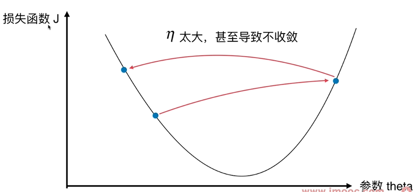
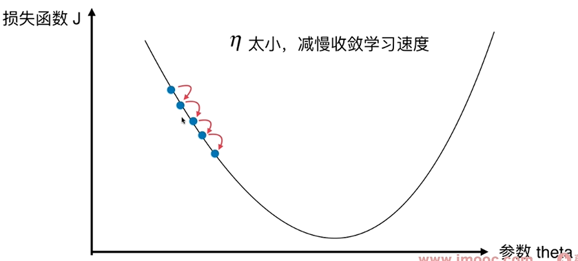
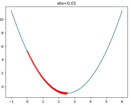
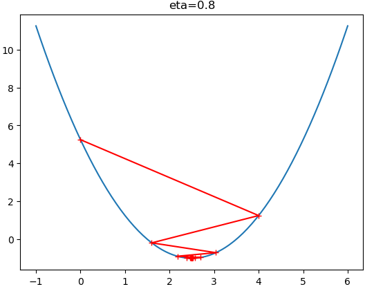
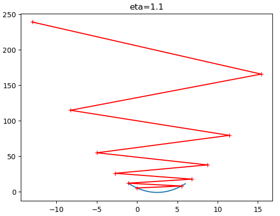
$\eta$ 值会影响算法能否快速收敛:
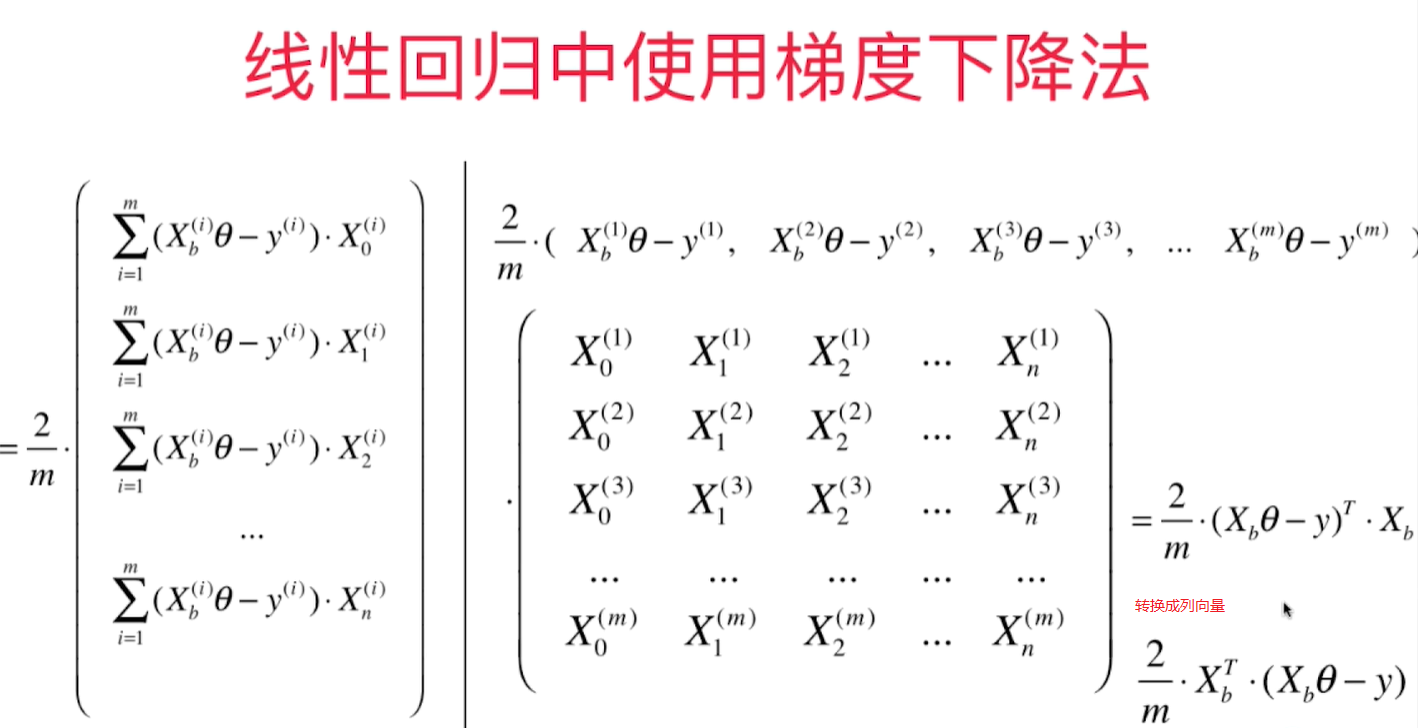
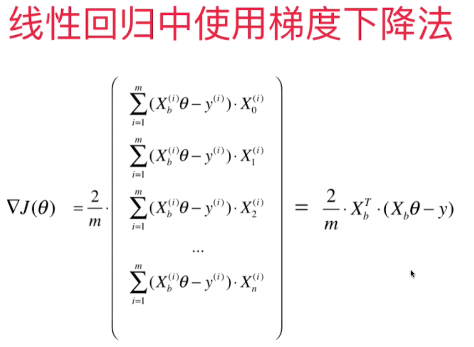
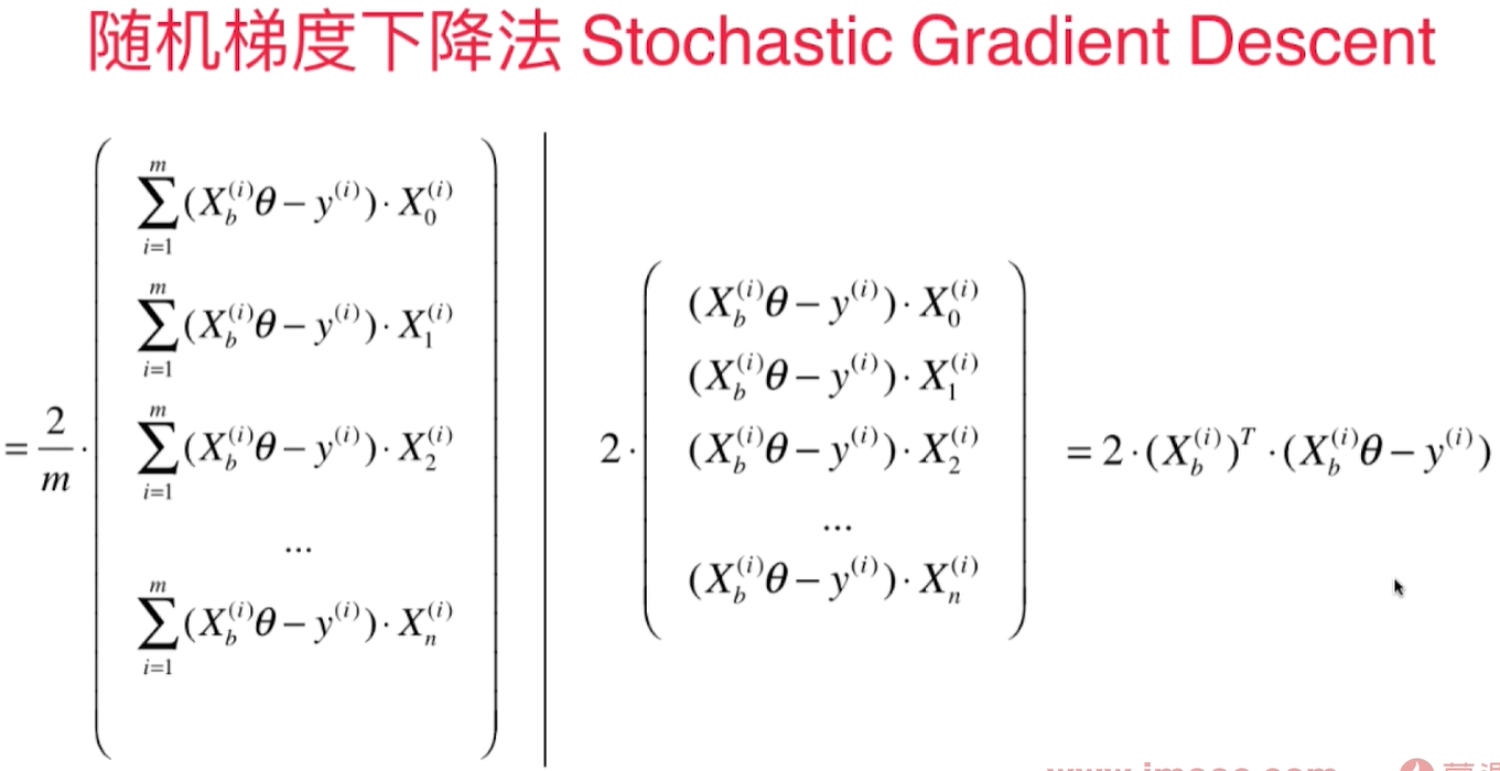
线性回归中的梯度下降法
对于高维样本,梯度代表的方向,就是J增大最快的方向。梯度就是对各个参数的偏导数.
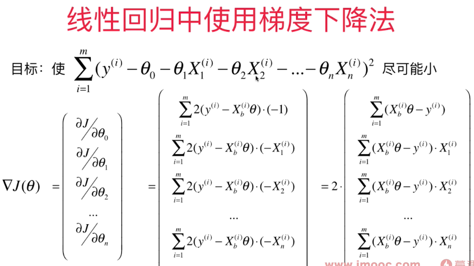
梯度大小和样本数量有关,梯度越大,样本中每个元素的梯度也越大。 - 最佳的: 每一个梯度值和样本个数无关。所以要在求出的梯度值除以m。
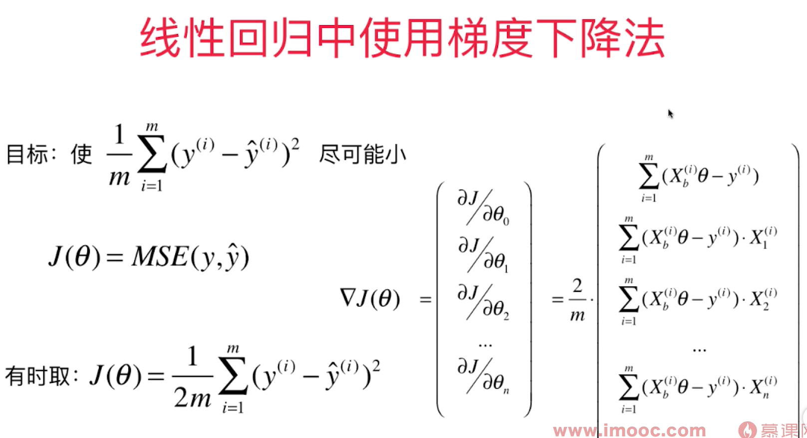
目标函数变成了求MSE
实现线性回归中的梯度下降法
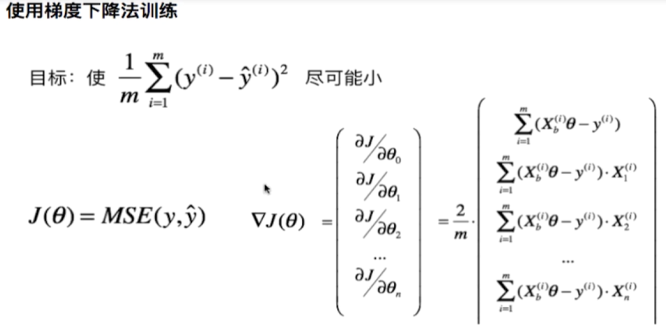
在LinearRegression类中实现了fit_gd函数:
    def fit_gd(self, X_train, y_train):
        assert X_train.shape[0] == y_train.shape[0], "The X_train's size should be equal to the y_train's size"
        def dJ(theta, X_b, y):
            gd = np.zeros_like(theta)
            for i in range(len(theta)):
                if i == 0:
                    gd[0] = np.sum((X_b.dot(theta) - y))
                else:
                    gd[i] = np.sum((X_b.dot(theta) - y).dot(X_b[:, i]))
            return gd * 2 / len(X_b)

        def J(theta, X_b, y):
            try:
                return np.sum((X_b.dot(theta) - y) ** 2) * 2 / len(X_b)
            except:
                return float('inf')

        def gradient_descent(X_b, y, initial_theta, eta, n_iters=1e4, epsilon=1e-8):
            theta = initial_theta
            i_iter = 0

            while (i_iter < n_iters):
                last_theta = theta
                gradient = dJ(theta, X_b, y)
                theta = theta - eta*gradient
                if np.abs(J(theta, X_b, y) - J(last_theta, X_b, y)) < epsilon:
                    break
                i_iter += 1
            return theta

        X_b = np.hstack((np.ones((len(X_train), 1)), X_train))
        initial_theta = np.zeros(X_b.shape[1])
        eta = 0.01
        self._theta = gradient_descent(X_b, y_train, initial_theta, eta)
        self.coef_ = self._theta[1:]
        self.intercept_ = self._theta[0]
        return self
测试代码:
import numpy as np
import matplotlib.pyplot as plt
import sys
sys.path.append(r'C:\\N-20KEPC0Y7KFA-Data\\junhuawa\\Documents\\00-Play-with-ML-in-Python\\Jupyter')
import playML
from playML.LinearRegression import LinearRegression
lin_reg = LinearRegression()
np.random.seed(666)
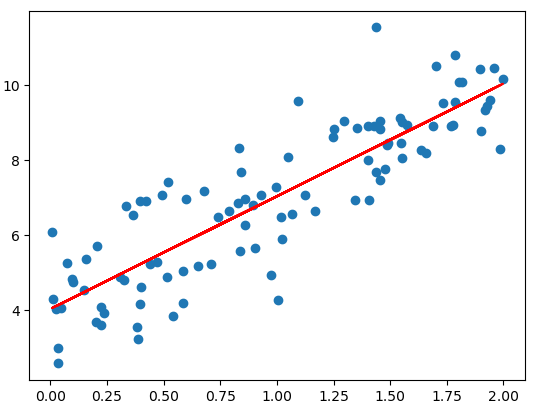
x = 2*np.random.random(size=100)
y = x*3. + 4. + np.random.normal(size=100)
X = x.reshape(-1, 1)
lin_reg.fit_gd(X, y)
y_predict = x*lin_reg.coef_ + lin_reg.intercept_
plt.scatter(x, y)
plt.plot(x, y_predict, color='r')
lin_reg._theta
array([4.06880601, 3.08632808])
梯度下降法的向量化和数据标准化
用向量运算代替for循环
在Numpy里,一个向量默认都是列向量,要转换成行向量需要转置。但是Numpy里对于行,列向量的运算是一样的,不做区分。
上一节求梯度的方法可以转换成简洁的矩阵运算:
        def dJ(theta, X_b, y):
            gd = np.zeros_like(theta)
            for i in range(len(theta)):
                if i == 0:
                    gd[0] = np.sum((X_b.dot(theta) - y))
                else:
                    gd[i] = np.sum((X_b.dot(theta) - y).dot(X_b[:, i]))
            return gd * 2 / len(X_b)
转换为:
        def dJ(theta, X_b, y):
            return X_b.T.dot(X_b.dot(theta) - y) * 2. / len(X_b)
最终的代码fit_gd()如下:
    def fit_gd(self, X_train, y_train, eta = 0.1, n_iters=1e4):
        assert X_train.shape[0] == y_train.shape[0], "The X_train's size should be equal to the y_train's size"
        def dJ(theta, X_b, y):
            #         res = np.zeros_like(theta)
            #        gd = np.zeros_like(theta)

            #        for i in range(len(theta)):
            #            if i == 0:
            #                gd[0] = np.sum((X_b.dot(theta) - y))
            #            else:
            #               gd[i] = np.sum((X_b.dot(theta) - y).dot(X_b[:, i]))
            #        return gd * 2 / len(X_b)
            return X_b.T.dot(X_b.dot(theta) - y) * 2. / len(X_b)


        def J(theta, X_b, y):
            try:
                return np.sum((X_b.dot(theta) - y) ** 2) / len(X_b)
            except:
                return float('inf')

        def gradient_descent(X_b, y, initial_theta, eta, n_iters, epsilon=1e-8):
            theta = initial_theta
            i_iter = 0

            while (i_iter < n_iters):
                last_theta = theta
                gradient = dJ(theta, X_b, y)
                theta = theta - eta*gradient
                if np.abs(J(theta, X_b, y) - J(last_theta, X_b, y)) < epsilon:
                    break
                i_iter += 1
            return theta

        X_b = np.hstack((np.ones((len(X_train), 1)), X_train))
        initial_theta = np.zeros(X_b.shape[1])
        self._theta = gradient_descent(X_b, y_train, initial_theta, eta, n_iters)
        self.coef_ = self._theta[1:]
        self.intercept_ = self._theta[0]
        return self
boston房价数据读取和regression类加载:
import numpy as np
from sklearn import datasets
import matplotlib.pyplot as plt
import pandas as pd
data= pd.read_csv("boston_house_prices.csv", skiprows=[0])
array = data.values
X = array[:, :13]
y = array[:, 13]
import sys
sys.path.append(r'C:\\N-20KEPC0Y7KFA-Data\\junhuawa\\Documents\\00-Play-with-ML-in-Python\\Jupyter')
import playML
from playML.model_selection import train_test_split
X_train, X_test, y_train, y_test = train_test_split(X, y, seed=666)
from playML.LinearRegression import LinearRegression
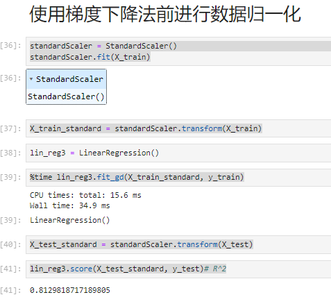
数据归一化
在真实数据中,每一维的数据大小相差很大,导致需要步长尽可能小(0.000001),回归次数(1e6)尽可能多才能达到理想的模型, 但是这样也会导致收敛速度很慢,计算量很大的问题。为了达到理想的效果,需要对数据进行归一化。归一化后,算法效率提高很多。
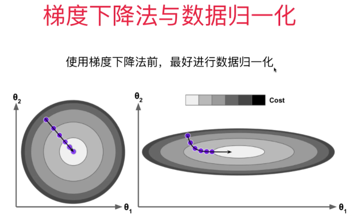
梯度下降法和线性回归法(正规方程法)的比较:
- 正规方程解法中不需要对数据做归一化,因为求解只是对矩阵的运算,没有搜索的过程。 在GD中,步长会受到各个维度数据的影响。数据归一化可以解决这个问题,数据归一化后,收敛速度大幅提高!
- 正规方程法需要对m*n的矩阵做大量的乘法运算( $O(n^3)$ ),矩阵大时效率低。
- 但是对于梯度下降法,如果样本数量m增大,因为每次都要对所有样本进行计算,效率也会降低,所以引出了随机梯度下降法。
from sklearn.preprocessing import StandardScaler
standardScaler = StandardScaler()
standardScaler.fit(X_train)
X_train_standard = standardScaler.transform(X_train)
lin_reg3 = LinearRegression()
%time lin_reg3.fit_gd(X_train_standard, y_train)
X_test_standard = standardScaler.transform(X_test)
lin_reg3.score(X_test_standard, y_test)# R^2
正规法和梯度下降法性能比较:
m = 1000
n = 5000
big_X = np.random.normal(size=(m, n))
true_theta = np.random.uniform(0.0, 100.0, size=n+1)
big_y = big_X.dot(true_theta[1:]) + true_theta[0]+np.random.normal(0.0, 10., size=m)

big_reg1 = LinearRegression()
%time big_reg1.fit_normal(big_X, big_y)

big_reg2 = LinearRegression()
%time big_reg2.fit_gd(big_X, big_y)
结果:
CPU times: total: 14.8 s
Wall time: 5.1 s
CPU times: total: 11 s
Wall time: 3.49 s
总结: 当特征值和样本量数量很大时,GD性能比LR好!,但对于GD来说,如果样本量增大,他的性能也会减少,所以引入随机梯度下降法。一次只用计算一个样本的梯度。
https://blog.csdn.net/hai411741962/article/details/132580367
随机梯度下降法 Stochastic Gradient Descent(SGD)
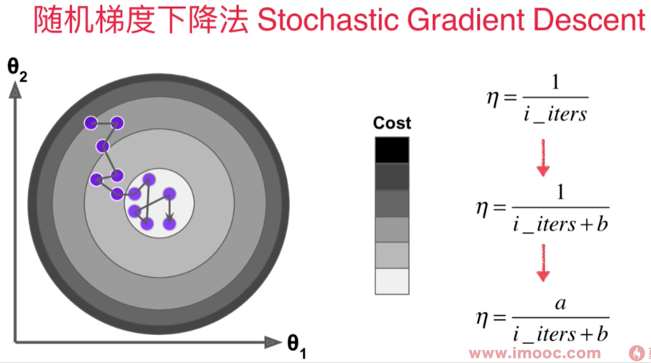
每次只取出第i个样本进行计算,得到的值决定了下一次的搜索方向,有可能往梯度增大的方向前进,但是总的来说会逼近最小值。尤其是当样本数m值很大时,我们愿意用精度换取时间。
为了避免我们已经到loss function的最小值附近,但是因为学习率过大,导致又跳出了最小值附近,我们希望学习率是逐渐递减的。 而这个逐渐递减的过程借用了搜索领域著名的模拟退火思想。 既在冶金的过程中,钢铁的温度是从高到低冷却的!冷却的函数是和时间t相关的。
用$1/3$的样本就可以得到较精确的结果:
import numpy as np
import matplotlib.pyplot as plt
m = 100000
x = np.random.normal(size=m)
X = x.reshape(-1, 1)
y = 4.*x + 3.+np.random.normal(0, 3, size=m)

def dJ_sgd(theta, X_b_i, y_i):
    return X_b_i.T.dot(X_b_i.dot(theta) - y_i) * 2.

def J(theta, X_b, y):
    try:
        return np.sum((X_b.dot(theta) - y) ** 2) / len(X_b)
    except:
        return float('inf')

def sgd(X_b, y, theta, n_iters):

    t0 = 5
    t1 = 50
    def learning_rate(t):
        return t0/(t + t1)

    for cur_iter in range(n_iters):
        rand_i = np.random.randint(len(X_b))
        gradient = dJ_sgd(theta, X_b[rand_i], y[rand_i])
        theta = theta - learning_rate(cur_iter) * gradient
    return theta

%%time
X_b = np.hstack([np.ones((len(X), 1)), X])
initial_theta = np.zeros(X_b.shape[1])
theta = sgd(X_b, y, initial_theta, len(X)//3)

theta
结果:
CPU times: total: 219 ms
Wall time: 368 ms
array([2.94080133, 4.02817242])
scikit-learn 中的随机梯度下降法
不需要从外部传递 $ \eta$,因为 $\eta$ 随着循环次数而变。
n_iters:代表对传入的所有的样本看几遍?比如5,看5遍,总的循环次数是n_iters*m
在每一遍遍历中,要对所有样本随机地看一遍。- 把所有样本先乱序排序,然后再从头开始取出每一个样本,这样就可以随机的把所有的样本看一遍。
indexes = np.random.permutation(m)
fit_sgd() 函数实现:
    def fit_sgd(self, X_train, y_train, n_iters=5, t0 = 5, t1=50): #n_iters代表要遍历几遍所有的样本
        assert X_train.shape[0] == y_train.shape[0], "The X_train's size should be equal to the y_train's size"
        assert n_iters >= 1, "所有的样本至少要看一遍"
        def learning_rate(t, t0, t1):
            return t0 / (t + t1)

        def dJ_sgd(theta, X_b_i, y_i):
            return X_b_i.T.dot(X_b_i.dot(theta) - y_i) * 2.

        def sgd(X_b, y, theta, n_iters, t0, t1):
            m = len(X_b)
            for cur_iter in range(n_iters):
                indexes = np.random.permutation(m)
                X_b_new = X_b[indexes] #通过fancy indexing获得新的array
                y_new = y[indexes]
                for i in range(m):
                    gradient = dJ_sgd(theta, X_b_new[i], y_new[i])
                    theta = theta - learning_rate(cur_iter*m + i, t0, t1) * gradient
            return theta

        X_b = np.hstack([np.ones((len(X_train), 1)), X_train])
        initial_theta = np.zeros(X_b.shape[1])
        self._theta = sgd(X_b, y_train, initial_theta, n_iters, t0, t1)
        self.coef_ = self._theta[1:]
        self.intercept_ = self._theta[0]
        return self
测试数据 boston 房价:
from sklearn import datasets
import matplotlib.pyplot as plt
import pandas as pd
data= pd.read_csv("boston_house_prices.csv", skiprows=[0])
array = data.values
X = array[:, :13]
y = array[:, 13]
X = X[y<50.0]
y = y[y<50.0]
测试训练数据集拆分:
from playML.model_selection import train_test_split
X_train, X_test, y_train, y_test = train_test_split(X, y, seed = 666)
对数据进行归一化处理:
from sklearn.preprocessing import StandardScaler
standardScaler = StandardScaler()
standardScaler.fit(X_train)
X_train_standard = standardScaler.transform(X_train)
X_test_standard = standardScaler.transform(X_test)
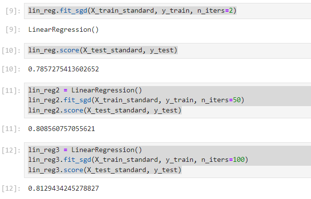
拟合并测试 $R^2$ Score:
from playML.LinearRegression import LinearRegression
lin_reg = LinearRegression()
lin_reg.fit_sgd(X_train_standard, y_train, n_iters=2)
lin_reg.score(X_test_standard, y_test)

lin_reg2 = LinearRegression()
lin_reg2.fit_sgd(X_train_standard, y_train, n_iters=50)
lin_reg2.score(X_test_standard, y_test)

lin_reg3 = LinearRegression()
lin_reg3.fit_sgd(X_train_standard, y_train, n_iters=100)
lin_reg3.score(X_test_standard, y_test)
scikit-learn中的SGD
from sklearn.linear_model import SGDRegressor
sgd_reg = SGDRegressor(max_iter=100)
sgd_reg.fit(X_train_standard, y_train)
sgd_reg.score(X_test_standard, y_test)
结果:
0.8122765915486065
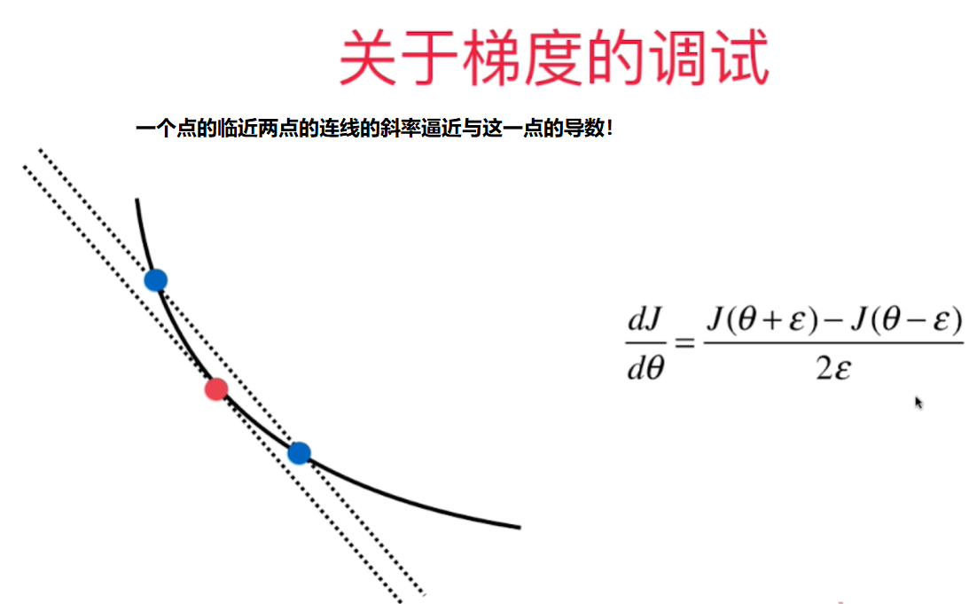
如何判断梯度下降法中梯度值是正确的?- 极限求导
Debug的时候,可以用极限求导的定义来算出梯度值(效率低),用来验证向量化矩阵运算获得的梯度值是否正确。
def J(theta, X_b, y):
try:
return np.sum((X_b.dot(theta) - y) ** 2) / len(X_b)
except:
return float('inf')
def dJ_math(theta, X_b, y): # 用矩阵运算求导
return X_b.T.dot(X_b.dot(theta) - y) * 2. / len(X_b)
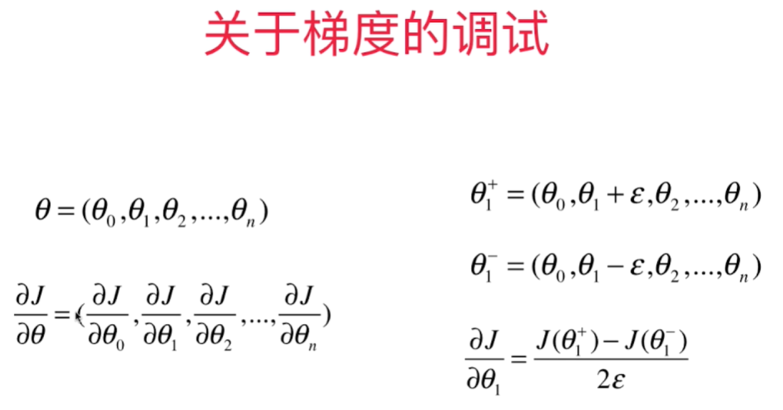
def dJ_debug(theta, X_b, y, epsilon=0.01): # 用极限方法求导
res = np.empty(len(theta))
for i in range(len(theta)):
theta_1 = theta.copy()
theta_2 = theta.copy()
theta_1[i] += epsilon
theta_2[i] -= epsilon
res[i] = (J(theta_1, X_b, y) - J(theta_2, X_b, y)) /(2*epsilon)
return res
# implemnented in playML.LinearRegression
def fit_gd_debug(self, dJ, X_train, y_train, n_iters=1e4):
assert X_train.shape[0] == y_train.shape[0], "The X_train's size should be equal to the y_train's size"
def gradient_descent(dJ, X_b, y, initial_theta, eta, n_iters, epsilon=1e-8):
theta = initial_theta
i_iter = 0
while (i_iter < n_iters):
last_theta = theta
gradient = dJ(theta, X_b, y)
theta = theta - eta*gradient
if np.abs(J(theta, X_b, y) - J(last_theta, X_b, y)) < epsilon:
break
i_iter += 1
return theta
X_b = np.hstack((np.ones((len(X_train), 1)), X_train))
initial_theta = np.zeros(X_b.shape[1])
eta=0.01
self._theta = gradient_descent(dJ, X_b, y_train, initial_theta, eta, n_iters)
self.coef_ = self._theta[1:]
self.intercept_ = self._theta[0]
return self
测试代码:
import numpy as np
import matplotlib.pyplot as plt
np.random.seed(666)
X=np.random.random(size=(1000,10))
true_theta = np.arange(1, 12, dtype=float)
X_b = np.hstack([np.ones((len(X), 1)), X])
y = X_b.dot(true_theta) + np.random.normal(size=1000)
import sys
sys.path.append(r'C:\\N-20KEPC0Y7KFA-Data\\junhuawa\\Documents\\00-Play-with-ML-in-Python\\Jupyter')
import playML
from playML.LinearRegression import LinearRegression

lin_reg1 = LinearRegression()
lin_reg1.fit_gd_debug(dJ_math, X, y)
lin_reg1._theta

lin_reg2 = LinearRegression()
lin_reg2.fit_gd_debug(dJ_debug, X, y)
lin_reg2._theta
小批量梯度下降法
批量梯度下降法 Batch Gradient Descent - 每次对所有样本做运算,效率低但是稳定,总是向损失函数下降的方向前进!
随机梯度下降法 Stochastic Gradient Descent - 计算速度快,但是不稳定,甚至有可能向反方向前进。
小批量梯度下降法 mini-batch Gradient Descent - 每次看K个样本,兼顾了速度,得到的梯度也比SGD稳定一些 - 超参数K
随机能帮我们跳出局部最优解。机器学习解决的是在不确定的世界中的不确定的问题。本身就没有一个固定的最优解!

PCA - 主成分分析 - Principal Component Analysis
研究生阶段的数理统计课程覆盖PCA。

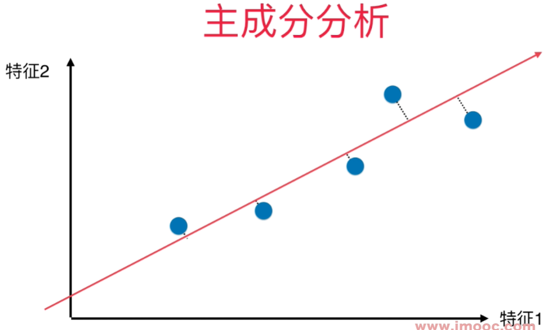
如何找到让样本间间距最大的轴 - 方差(Variance) - 描述整体样本疏密的指标, 大代表样本稀疏,小代表样本越紧密。
$$ \begin{aligned} Var(x) = \frac{1}{m}\sum_{i=1}^m(x_i - \overline x)^2 \end{aligned} $$
横轴纵轴代表两个特征,将2维平面降到1维平面,用一条线去拟合原来的那些点,这些映射到这条线上的点与原来的2维的样本点没有更大的差距。点和点之间的距离比原来将点映射到X轴或者Y轴都大,点之间的区分度也更加明显。
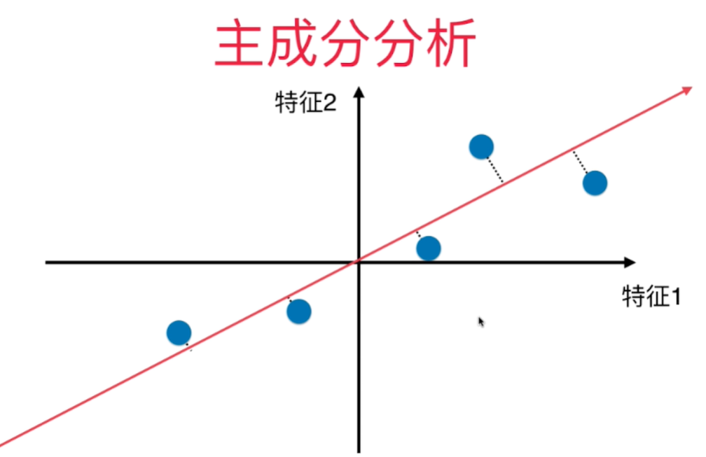
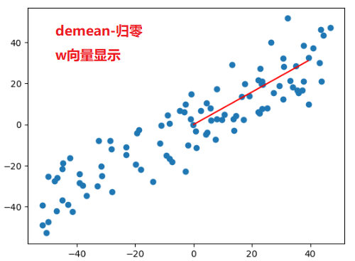
对所有的样本进行demean处理 - 归零 - 每个样本都减去样本均值. 坐标轴进行了移动,使得样本在每一个维度上的均值为0.
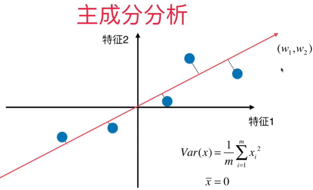
$X_i$ 是将原来的样本点映射到斜线(新的坐标轴)上之后得到的的新的样本值 $(w1, w2)$
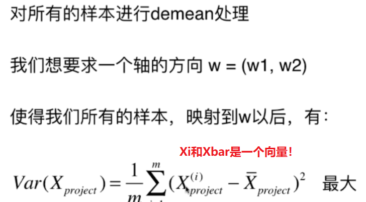
使2个向量相减之后的模的平方达到最大值
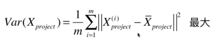
因为 $X_{project}$ 做过demean处理,均值为0, 所以
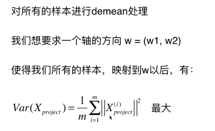
把所有的样本点映射到w轴上之后得到的新的样本点的模的平方和最大。
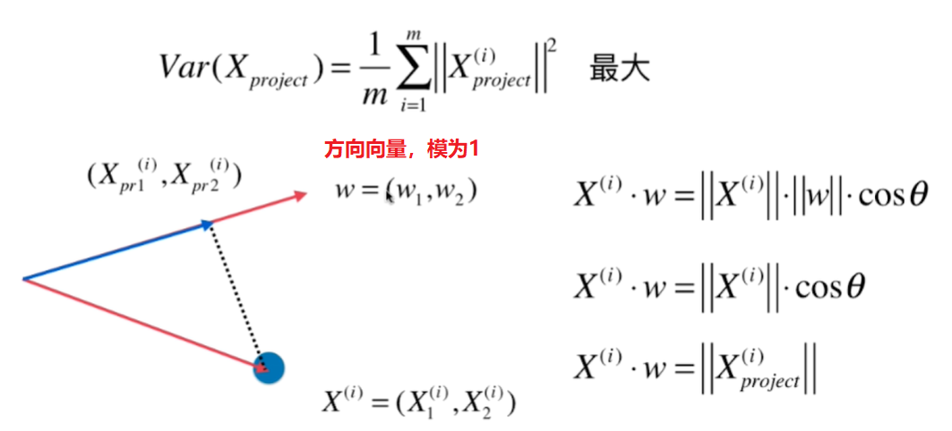
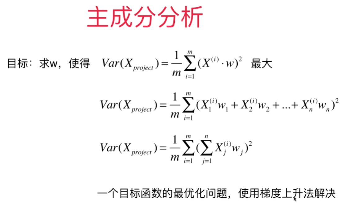
要求 $$Var(X_{project}) = \frac{1}{m} \sum^m_{i=1} {\Vert X^{(i)}\cdot w\Vert}^2$$ 最大!
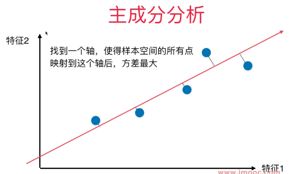
主成分分析法:找到一个轴,使得样本空间的所有点映射到这个轴后,方差最大。 所有的点的距离线垂直于找到的线。
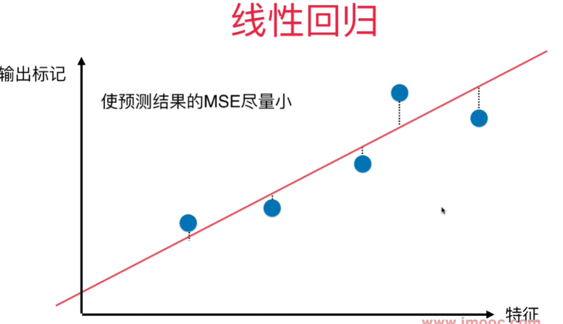
线性回归:找到一根直线,使的输出标记和所有在X轴上的特征值对应的直线上的点之间的MSE尽量小。这些距离线垂直于X轴。
两者都有样本和一根直线之间的关系,但是关系是不同的。
使用梯度上升法求解PCA问题
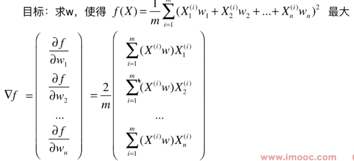
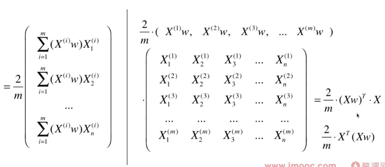
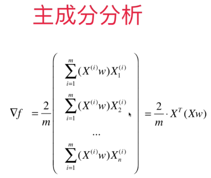
求出主成分分析法中的目标函数f和对应的梯度
求数据主成分PCA
求解梯度上升法的注意事项:
- 每一次都要求出w的一个单位方向向量,因为算法里要求的就是单位向量, 如果不用单位向量,搜索会不稳定。
- 初始搜索的w不能为0,要随机化一个向量。 为0的向量得到的梯度也为0.
- 不能使用standardScaler标准化数据, 如果先对数据进行标准化,则不是一个线性的变化,会影响数据的分布, 得到的主成分和原始的数据不一样。 demean只是把数据在坐标轴上进行位移,不影响数据的分布,所以可以操作。
我们通过PCA求得的这个单位向量(轴)就是第一个主成分。 PCA是一种无监督学习,因为算法中不需要y.
def demean(X):
   return X - np.mean(X, axis = 0)

def f(X, w):
   return np.sum(X.dot(w) ** 2) / len(X)

def df_math(X, w):
   return X.T.dot(X.dot(w)) * 2 / len(X)

def df_debug(X, w, epsilon=0.0001):  # w是一个方向向量,模为1,每个维度的值都很小, 所以epsilon的值也小
   res = np.empty(len(w))
   for i in range(len(w)):
       w_1 = w.copy()
       w_2 = w.copy()
       w_1[i] += epsilon
       w_2[i] -= epsilon
       res[i] = (f(X, w_1) - f(X, w_2)) / (2 * epsilon)
   return res

def direction(w):  # 求单位向量
   return w / np.linalg.norm(w)

def gradient_ascent(df, X, initial_w, eta, n_iters=1e4, epsilon=1e-8):
   w = direction(initial_w)
   i_iter = 0
   while (i_iter < n_iters):
       last_w = w
       gradient = df(X, w)
       w = w + eta * gradient
       w = direction(w)
       if np.abs(f(X, w) - f(X, last_w)) < epsilon:
           break
       i_iter += 1
   return w
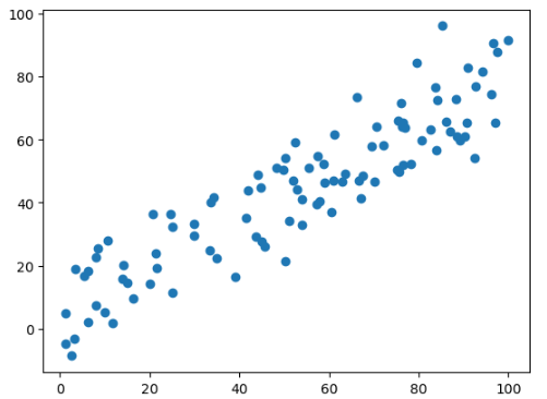
import numpy as np
import matplotlib.pyplot as plt
X = np.empty((100, 2))
X[:, 0] = np.random.uniform(0, 100, size=100)
X[:, 1] = 0.75*X[:, 0] + 3.0 + np.random.normal(0, 10, size=100)
def demean(X): #需要对原始数据做demean处理 - 归零
    return X - np.mean(X, axis = 0)
X_demean = demean(X)

initial_w = np.random.random(X.shape[1])
w = gradient_ascent(df_math, X_demean, initial_w, eta)

plt.scatter(X_demean[:, 0], X_demean[:, 1])
plt.plot((0, w[0] * 50), (0, w[1]*50), color='r')
求数据的前n个主成分
求出第一个主成分以后,如何求出下一个主成分呢?
- 将数据进行改变,将数据在第一个主成分上的分量去掉。
$X^{'(i)}$ 是X中去除第一个主成分上的分量之后剩下的结果。 求下一个主成分 - 将第一个主成分上的分量去掉,在新的数据上求第一个主成分
    def first_n_components(n, X, eta = 0.001, n_iters=1e4, epsilon=1e-8):

        def first_component(X, initial_w, eta=0.001, n_iters=1e4, epsilon=1e-8):
            def f(X, w):
                return np.sum(X.dot(w) ** 2) / len(X)

            def df(X, w):
                return X.T.dot(X.dot(w)) * 2 / len(X)

            def direction(w):  # 求单位向量
                return w / np.linalg.norm(w)

            w = direction(initial_w)
            i_iter = 0

            while (i_iter < n_iters):
                last_w = w
                gradient = df(X, w)
                w = w + eta * gradient
                w = direction(w)
                if np.abs(f(X, w) - f(X, last_w)) < epsilon:
                    break
                i_iter += 1
            return w

        def demean(X):  # 需要对原始数据做demean处理 - 归零
            return X - np.mean(X, axis=0)

        X_pca = X.copy()
        res = []
        X_pca = demean(X_pca)
        for i in range(n):
            initial_w = np.random.random(X_pca.shape[1])
            w = first_component(X_pca, initial_w)
            res.append(w)
            X_pca = X_pca - (X_pca.dot(w)).reshape(-1, 1) * w

        return res
向量化运算 - 将原样本减去映射到w方向上的分量
X2 = np.empty(X.shape)
#for i in range(len(X)):
#    X2[i] = X[i] - X[i].dot(w)*w #点乘得到向量的模,然后再乘上单位向量得到X[i]在w方向上的分量。
X2 = X - (X.dot(w)).reshape(-1, 1)*w #X.dot(w)得到一个向量,将向量转换为m*1维的矩阵,然后于w相乘,就是把模乘上单位向量,得到每个样本在这个单位向量上的分量。
测试代码:
import numpy as np
import matplotlib.pyplot as plt
import sys
sys.path.append(r'C:\\N-20KEPC0Y7KFA-Data\\junhuawa\\Documents\\00-Play-with-ML-in-Python\\Jupyter')
import playML
from playML.pca import PCA
pca = PCA()
X = np.empty((100, 2))
X[:, 0] = np.random.uniform(0, 100, size=100)
X[:, 1] = 0.75*X[:, 0] + 3.0 + np.random.normal(0, 10, size=100)
w = PCA.first_n_components(2, X)
w
w[0].dot(w[1]) # 单位向量正交,点积为0
结果:
[array([0.7694744 , 0.63867765]), array([ 0.63870067, -0.7694553 ])]
2.991102889515762e-05
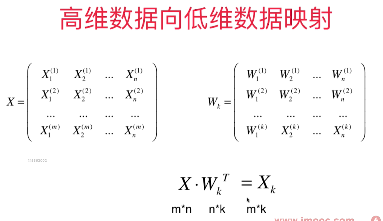
高维数据向低维数据映射
k 个主成分,每个主成分都是n维的。主成分分析的目的就是把样本从一个坐标系转换到另一个坐标系。 我们只取出前k个主成分(每个主成分的坐标轴有n个元素),因为这个前k个特征特别重要。形成W这个矩阵,这个矩阵是k*n的。
样本1和k个W相乘的结果就是样本1映射到 $W_k$ 这个坐标系上得到的k维的向量。 k 比n小,所以完成了一个样本从n维到k维(高维向低维)的映射。
高维向低维映射
也可以从低维恢复到高维,但是降维时丢失的信息无法恢复
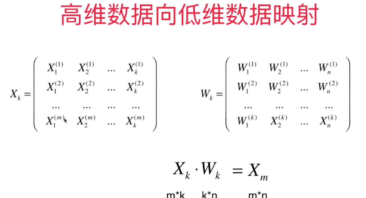
求出k个主成分得到$W_k$这个矩阵,得到K个轴的单位方向向量之后,就可以从高维向低维数据的映射,也可以反过来从低维映射回高维数据。
封装的PCA类包含fit, transform, inverse_transform 函数:
import numpy as np

class PCA:
    def __init__(self, n_components):
        """初始化PCA模型"""
        assert n_components >= 1, "n_components must be bigger than 0."
        self.n_components = n_components
        self.components_ = None

    def fit(self, X, eta = 0.01, n_iters = 1e4):
        assert self.n_components <= X.shape[1], "n_components must be not bigger than the feature number of X."
        def f(X, w):
            return np.sum(X.dot(w) ** 2) / len(X)
        def df(X, w):
            return X.T.dot(X.dot(w)) * 2 / len(X)
        def direction(w):  # 求单位向量
            return w / np.linalg.norm(w)
        def demean(X):  # 需要对原始数据做demean处理 - 归零
            return X - np.mean(X, axis=0)
        def first_component(X, initial_w, eta=0.001, n_iters=1e4, epsilon=1e-8):
            w = direction(initial_w)
            i_iter = 0
            while (i_iter < n_iters):
                last_w = w
                gradient = df(X, w)
                w = w + eta * gradient
                w = direction(w)
                if np.abs(f(X, w) - f(X, last_w)) < epsilon:
                    break
                i_iter += 1
            return w

        X_pca = demean(X)
        self.components_ = np.empty(shape=(self.n_components, X.shape[1]))
        for i in range(self.n_components):
            initial_w = np.random.random(X_pca.shape[1])
            w = first_component(X_pca, initial_w)
            self.components_[i, :] = w
            X_pca = X_pca - (X_pca.dot(w)).reshape(-1, 1) * w
        return self

    def transform(self, X):
        """将给定的X映射到各主成分分量中"""
        assert self.components_.shape[1] == X.shape[1], "n_components must be equal to the feature number of X."
        return X.dot(self.components_.T)

    def inverse_transform(self, X_k):
        """将给定的X_k反向映射到原来的特征空间"""
        assert self.components_.shape[0] == X_k.shape[1], "n_components must be equal to the feature number of X_k."
        return X_k.dot(self.components_)
    def first_n_components(n, X, eta = 0.001, n_iters=1e4, epsilon=1e-8):

        def first_component(X, initial_w, eta=0.001, n_iters=1e4, epsilon=1e-8):
            def f(X, w):
                return np.sum(X.dot(w) ** 2) / len(X)

            def df(X, w):
                return X.T.dot(X.dot(w)) * 2 / len(X)

            def direction(w):  # 求单位向量
                return w / np.linalg.norm(w)

            w = direction(initial_w)
            i_iter = 0

            while (i_iter < n_iters):
                last_w = w
                gradient = df(X, w)
                w = w + eta * gradient
                w = direction(w)
                if np.abs(f(X, w) - f(X, last_w)) < epsilon:
                    break
                i_iter += 1
            return w

        def demean(X):  # 需要对原始数据做demean处理 - 归零
            return X - np.mean(X, axis=0)

        X_pca = X.copy()
        res = []
        X_pca = demean(X_pca)
        for i in range(n):
            initial_w = np.random.random(X_pca.shape[1])
            w = first_component(X_pca, initial_w)
            res.append(w)
            X_pca = X_pca - (X_pca.dot(w)).reshape(-1, 1) * w

        return res

    def __repr__(self):
        return "PCA(n_components = %d)" % self.n_components
测试代码:
import numpy as np
import matplotlib.pyplot as plt
import sys
sys.path.append(r'C:\\N-20KEPC0Y7KFA-Data\\junhuawa\\Documents\\00-Play-with-ML-in-Python\\Jupyter')
import playML
from playML.pca import PCA
X = np.empty((100, 2))
X[:, 0] = np.random.uniform(0, 100, size=100)
X[:, 1] = 0.75*X[:, 0] + 3.0 + np.random.normal(0, 10, size=100)
pca = PCA(n_components = 1)
pca.fit(X)
X_reduction = pca.transform(X)
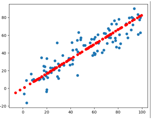
X_restore = pca.inverse_transform(X_reduction)
X_restore.shape
plt.scatter(X[:, 0], X[:, 1])
plt.scatter(X_restore[:, 0], X_restore[:, 1], color='r')
虽然恢复成2维的样本数据,但是显然他的原始数据信息已经丢失了。
scikit-learn中的PCA
scikit-learn中的PCA不是通过梯度上升法求解,而是用其他数学方法求的,所以求出的主成分方向和梯度上升法得到的不一样,但不影响降维结果。
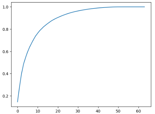
**pca.explained_variance_ratio_**解释的方差相应的比例
array([0.14566817, 0.13735469])
第一个轴可以解释14%的源数据的方差,第二个轴可以解释13%的源数据的方差。 用这个数组可以画出前k个主成分包含信息的多少:
from sklearn.decomposition import PCA
import numpy as np
from sklearn import datasets
digits = datasets.load_digits()
X = digits.data
y = digits.target
from sklearn.model_selection import train_test_split
X_train, X_test, y_train, y_test = train_test_split(X, y, random_state=666)
pca = PCA(X.shape[1])
pca.fit(X_train)
import matplotlib.pyplot as plt
plt.plot([i for i in range(X_train.shape[1])], [np.sum(pca.explained_variance_ratio_[:i+1]) for i in range(X_train.shape[1])])
可以往PCA构造函数中传入期望保留的信息比率,然后倒推主成分的数量:
pca = PCA(0.95)# 不知道要取多少个主成分,但是期望能得到95%的方差,也即能保留样本95%的信息
pca.fit(X_train)
pca.n_components_
结果: 28
用降维(64维降到28维)后的样本做分类得到的score, 速度也提高了一个数量级:
from sklearn.decomposition import PCA
import numpy as np
from sklearn.model_selection import train_test_split
X_train, X_test, y_train, y_test = train_test_split(X, y, random_state=666)
pca = PCA(0.95)# 不知道要取多少个主成分,但是期望能得到95%的方差,也即能保留样本95%的信息
pca.fit(X_train)
X_train_reduction = pca.transform(X_train)
X_test_reduction = pca.transform(X_test)
%%time
knn_clf_pca = KNeighborsClassifier()
knn_clf_pca.fit(X_train_reduction, y_train)
knn_clf_pca.score(X_test_reduction, y_test)
Result: CPU times: total: 625 ms Wall time: 150 ms 0.98
MNIST 数据集
当我们对原来样本做主成分分析降维后,准确率反而提高了 - 降噪 - 将原有的数据中的噪音消除了。 数据的维度减少,存储空间减少了,数据训练,预测的时间都减少了,预测准确率却提高了. - 降维的过程中把数据的噪音也消除了.
因为mnist数据集中的样本各个特征都是图像的像素点的数值,尺度是相同的,所以可以不用进行归一化处理。当各个维度尺度不同时,归一化是有意义的,把他们放在同样的尺度上在做拟合。
import numpy as np
from sklearn import datasets
from scipy.io import loadmat
mnist_data = loadmat('mnist-original.mat')
X, y = mnist_data['data'].T, mnist_data['label'].T
X_train = np.array(X[:60000], dtype=float)
y_train = np.array(y[:60000], dtype=float)
X_test, y_test = np.array(X[60000:], dtype=float), np.array(y[60000:], dtype=float)
y_train, y_test =  np.squeeze(y_train), np.squeeze(y_test)
from sklearn.neighbors import KNeighborsClassifier
knn_clf = KNeighborsClassifier()
%time knn_clf.fit(X_train, y_train)
%time knn_clf.score(X_test, y_test)
结果:
CPU times: total: 62.5 ms
Wall time: 68 ms
CPU times: total: 1min 15s
Wall time: 12.3 s
0.9688
from sklearn.decomposition import PCA
pca = PCA(0.9)
%time pca.fit(X_train)
pca.n_components_ #保留90%的信息,可以将数据从784维降到87维,降维幅度非常可观
X_train_reduction = pca.transform(X_train)
X_test_reduction = pca.transform(X_test)
knn_clf_pca = KNeighborsClassifier()
knn_clf_pca.fit(X_train_reduction, y_train)
%time knn_clf_pca.score(X_test_reduction, y_test)
结果:
CPU times: total: 16.5 s
Wall time: 6.89 s
CPU times: total: 17.7 s
Wall time: 3.17 s
0.9728
Scikit-Learn 中的多项式回归和Pipeline
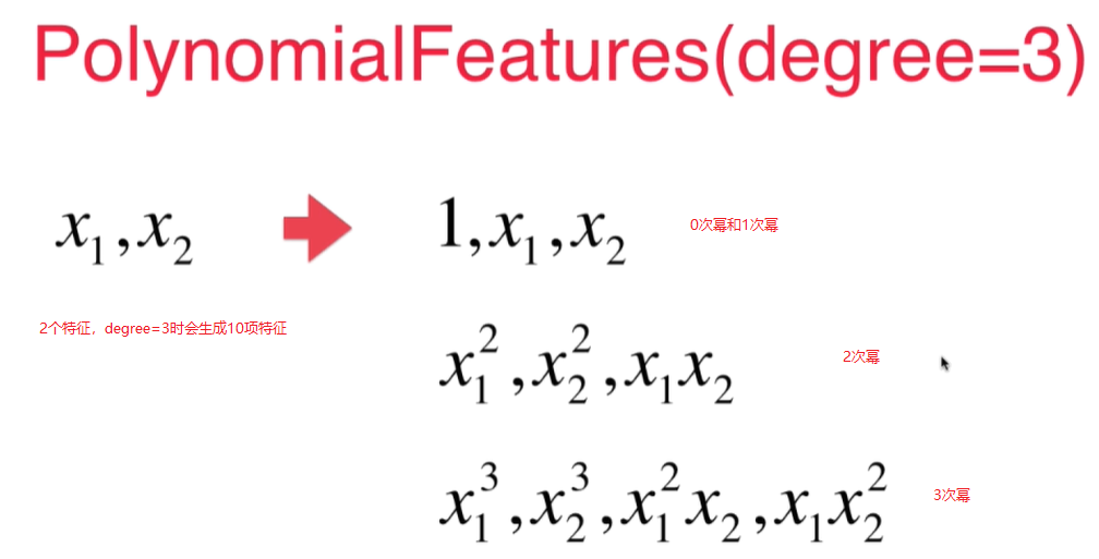
对于2次幂的特征,如果原本有 $x_1$, $x_2$ 2个特征的话, 最终会生成3列二次幂的特征!${x_1}^2$, $x_2^2$, $x_1$ * $x_2$ 这样3个特征, 经过transform之后生成了6个特征(原来的2个特征加上0次幂的特征,和生成的3个特征).
传入的degree=i时,经过多项式拟合后会生成 <= i的所有的项, 特征成指数级增长.
手动创建PolynomialFeatures类
import numpy as np
import matplotlib.pyplot as plt
from sklearn.preprocessing import PolynomialFeatures
x = np.random.uniform(-3, 3, size=100)
X = x.reshape(-1, 1)
y = 0.5*x**2 + x+2+np.random.normal(0, 1, 100)
poly = PolynomialFeatures(degree=2)
poly.fit(X)
X2 = poly.transform(X)
X2[:5,:] #X2的前5行
X[:5, :]**2
下面输出结果可见: - 第一列是x的0次幂的特征 - 第二列是x的1次幂的特征值 - 第三列是x的二次幂的特征值
array([[ 1.        ,  2.06105838,  4.24796164],
       [ 1.        ,  0.80578448,  0.64928863],
       [ 1.        , -2.95353343,  8.7233597 ],
       [ 1.        , -1.18450125,  1.40304321],
       [ 1.        ,  0.6798243 ,  0.46216109]])
array([[4.24796164],
       [0.64928863],
       [8.7233597 ],
       [1.40304321],
       [0.46216109]])
拟合
from sklearn.linear_model import LinearRegression
lin_reg2 = LinearRegression()
lin_reg2.fit(X2, y)
y_predict2 = lin_reg2.predict(X2)
plt.scatter(x, y)
plt.plot(np.sort(x), y_predict2[np.argsort(x)], color='r')
lin_reg2.coef_
lin_reg2.intercept_
输出结果:
array([0.        , 0.9887805 , 0.47970716])
2.0822081391267404
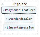
Pipeline
如果数据大小相差比较大,经过多项式回归会放大这个差距,所以需要用scalar先做归一化,再送给线性回归。
使用pipeline可以很方便的创建多项式回归这样一个类,这个类sklearn没有提供。
import numpy as np
import matplotlib.pyplot as plt
from sklearn.preprocessing import PolynomialFeatures
x = np.random.uniform(-3, 3, size=100)
X = x.reshape(-1, 1)
y = 0.5*x**2 + x+2+np.random.normal(0, 1, 100)
from sklearn.pipeline import Pipeline
from sklearn.preprocessing import StandardScaler
from sklearn.linear_model import LinearRegression
poly_reg = Pipeline([
("poly", PolynomialFeatures(degree=2)),
("std_scaler", StandardScaler()),
("lin_reg", LinearRegression())
])
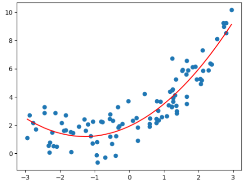
poly_reg.fit(X, y)
y_predict = poly_reg.predict(X)
plt.scatter(x, y)
plt.plot(np.sort(x), y_predict[np.argsort(x)], color='r')
结果:
归一化和未归一化得到的斜率和截距不一样
import numpy as np
import matplotlib.pyplot as plt
from sklearn.preprocessing import PolynomialFeatures
from sklearn.linear_model import LinearRegression
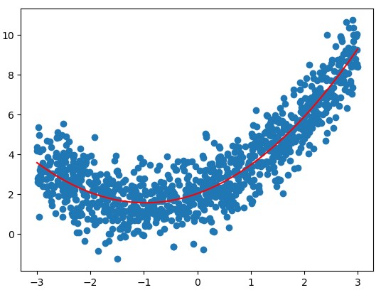
x = np.random.uniform(-3, 3, size=1000)
X = x.reshape(-1, 1)
y = 0.5*x**2 + x+2+np.random.normal(0, 1, 1000)
poly = PolynomialFeatures(degree=2)
poly.fit(X)
X2 = poly.transform(X)
stdscalar = StandardScaler()
stdscalar.fit(X2)
std_X2 = stdscalar.transform(X2)
lin_reg2 = LinearRegression()
lin_reg2.fit(std_X2, y)
y2 = lin_reg2.predict(std_X2)
plt.scatter(x, y)
plt.plot(np.sort(x), y2[np.argsort(x)], color='r')
lin_reg2.coef_
lin_reg2.intercept_
array([0.        , 1.65391099, 1.29661475])
3.485295640277668
过拟合与欠拟合 (Underfitting-and-overfitting)
均方误差
数据越高维 (度为10 或者100或者更高),拟合效果越好。可以找到一条曲线,将所有的样本点拟合进这条曲线(所有的样本点都在这条曲线上),均方误差为0,但是不是我们想要的, 曲线变得太过复杂了。 他可能不能反映我们样本的真实趋势。 Overfitting - 过拟合
用直线拟合数据,没有反应原始数据的样本特征 欠拟合 - underfitting
用pipeline得出度为2,10,100的时候的预测曲线:
测试用例:
import numpy as np
import matplotlib.pyplot as plt
from sklearn.linear_model import LinearRegression
np.random.seed(666)
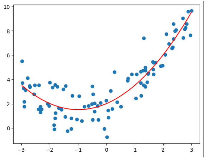
x = np.random.uniform(-3, 3, size=100)
X = x.reshape(-1, 1)
y = 0.5*x**2 + x + 2 + np.random.normal(0, 1, size=100)
Pipeline:
from sklearn.pipeline import Pipeline
from sklearn.preprocessing import PolynomialFeatures
from sklearn.preprocessing import StandardScaler

def PolynomialRegression(degree):
	return Pipeline([
		("poly", PolynomialFeatures(degree = degree)),
		("std_scaler", StandardScaler()),
		("lin_reg", LinearRegression())
		])
#degree = 2
poly_reg2 = PolynomialRegression(2)
poly_reg2.fit(X, y)
y_predict2 = poly_reg2.predict(X)
plt.scatter(x, y)
plt.plot(np.array(np.sort(x)), y_predict2[np.argsort(x)], color='r')
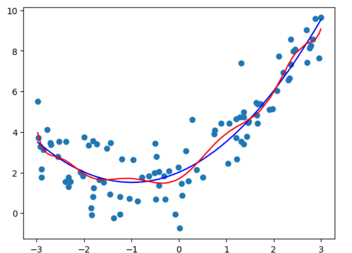
#degree = 10
poly_reg10 = PolynomialRegression(10)
poly_reg10.fit(X, y)
y_predict10 = poly_reg10.predict(X)
plt.scatter(x, y)
plt.plot(np.array(np.sort(x)), y_predict2[np.argsort(x)], color='b')
plt.plot(np.array(np.sort(x)), y_predict10[np.argsort(x)], color='r')
# degree = 100
poly_reg100 = PolynomialRegression(100)
poly_reg100.fit(X, y)
y_predict100 = poly_reg100.predict(X)
plt.scatter(x, y)
plt.plot(np.array(np.sort(x)), y_predict2[np.argsort(x)], color='b')
plt.plot(np.array(np.sort(x)), y_predict100[np.argsort(x)], color='r')
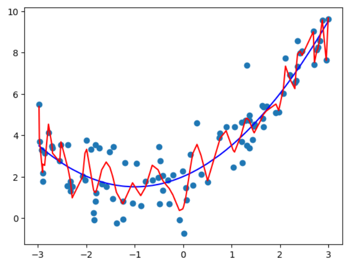
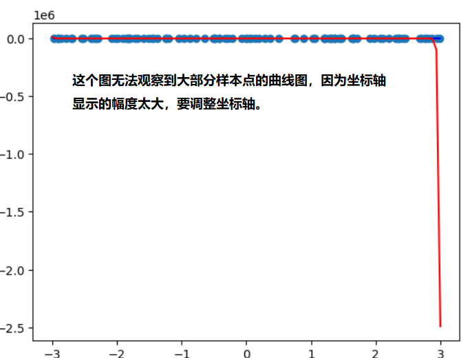
因为$x$数组的值不是均匀分布的,所以对于100度的真实曲线不是上图所示的,为了显示出真实的曲线,需要用均匀分布的x来画:
new_x = np.linspace(-3, 3, 100)
X_new = new_x.reshape(-1, 1)
y_new_100 = poly_reg100.predict(X_new)
plt.scatter(x, y)
plt.plot(np.array(np.sort(x)), y_predict2[np.argsort(x)], color='b')
plt.plot(np.array(X_new[:, 0]), y_new_100, color='r')
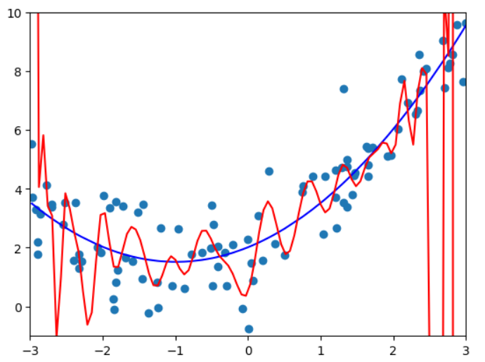
调整坐标轴后的结果:
plt.scatter(x, y)
plt.plot(np.array(np.sort(x)), y_predict2[np.argsort(x)], color='b')
plt.plot(np.array(X_new[:, 0]), y_new_100, color='r')
plt.axis([-3, 3, -1, 10])
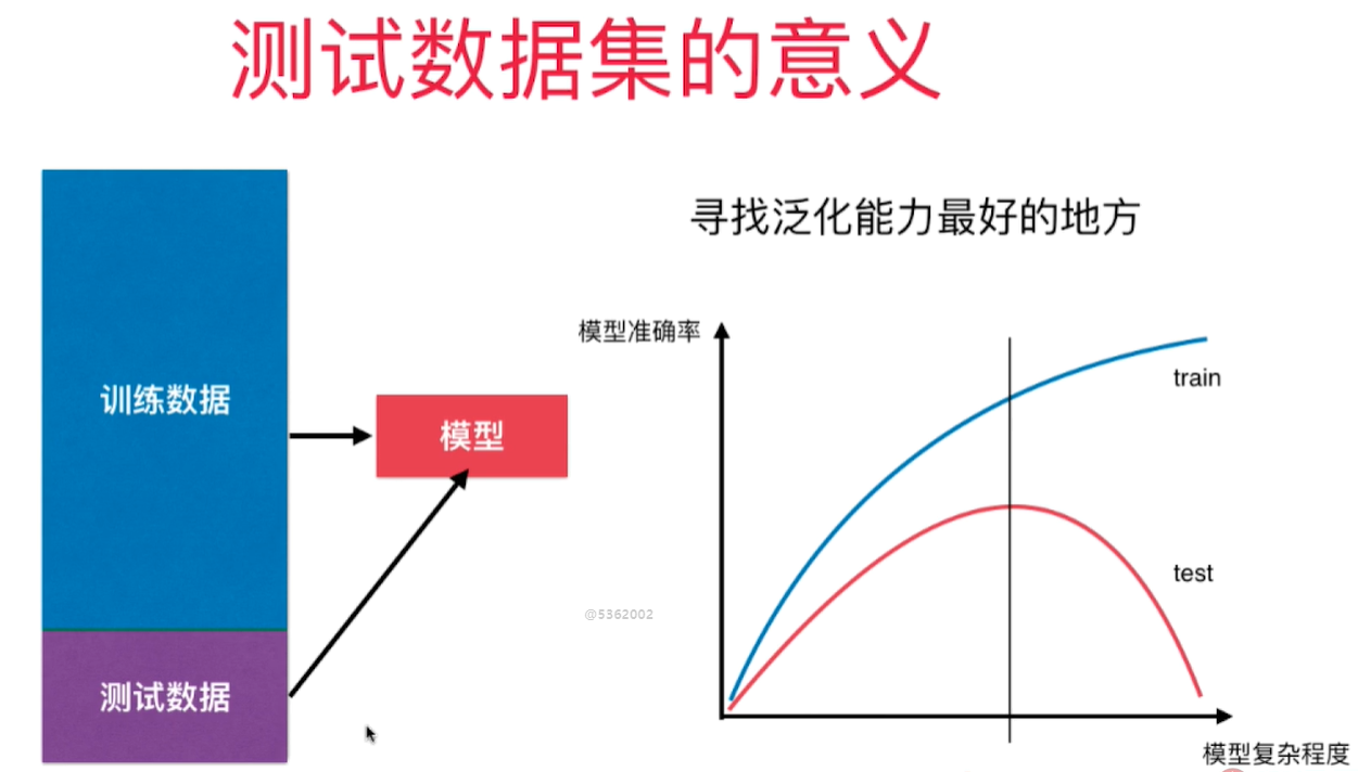
训练数据集和测试数据集
机器学习主要解决过拟合问题。 过拟合情况下,原有样本点拟合的很好,但是新样本点却不能很好的预测。 - 模型的泛化能力差 - 由此及彼的能力差(面对新样本的时候能力差)
要得到好的泛化能力 - 需要训练测试数据集的分离 - 对测试数据结果好的话则泛化能力强,否则则有可能遭遇了过拟合。
用训练得到的模型获得测试数据集的样本的预测值,然后和测试数据集的原标签值做均方差 - mean squared error
- 过拟合 overfitting - 算法所训练的模型过多的表达了数据间的噪音关系。
- 欠拟合 underfitting - 算法所训练的模型不能完整表述数据关系
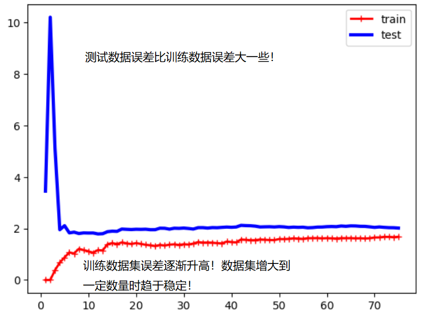
学习曲线
表示随着训练样本的逐渐增多,算法训练出的模型的表现能力。 测试数据:
import numpy as np
import matplotlib.pyplot as plt
from sklearn.linear_model import LinearRegression
np.random.seed(666)
x = np.random.uniform(-3, 3, size=100)
X = x.reshape(-1, 1)
y = 0.5*x**2 + x + 2 + np.random.normal(0, 1, size=100)
线性回归学习曲线绘制:
from sklearn.metrics import mean_squared_error
from sklearn.model_selection import train_test_split

def plot_learning_curves(X, y):
    #X_train, X_test, y_train, y_test = train_test_split(X, y, test_size=0.2)
    X_train, X_test, y_train, y_test = train_test_split(X, y, random_state=10)
    train_errors, test_errors = [], []
    for m in range(1, len(X_train)+1):
        model = LinearRegression()
        model.fit(X_train[:m], y_train[:m])
        y_train_predict = model.predict(X_train[:m])
        y_test_predict = model.predict(X_test)
        train_errors.append(mean_squared_error(y_train[:m], y_train_predict))
        test_errors.append(mean_squared_error(y_test, y_test_predict))
    plt.plot([i for i in range(1, len(X_train)+1)], np.sqrt(train_errors), 'r-+', linewidth=2, label="train")
    plt.plot([i for i in range(1, len(X_train)+1)], np.sqrt(test_errors), 'b-', linewidth=3, label="test")
    plt.legend()
plot_learning_curves(X, y)
 多项式回归学习曲线绘制:
def plot_learning_curves_with_algo(X, y, algo= LinearRegression()):
    #X_train, X_test, y_train, y_test = train_test_split(X, y, test_size=0.2)
    X_train, X_test, y_train, y_test = train_test_split(X, y, random_state=10)
    train_errors, test_errors = [], []
    for m in range(1, len(X_train)+1):
        algo.fit(X_train[:m], y_train[:m])
        y_train_predict = algo.predict(X_train[:m])
        y_test_predict = algo.predict(X_test)
        train_errors.append(mean_squared_error(y_train[:m], y_train_predict))
        test_errors.append(mean_squared_error(y_test, y_test_predict))
    plt.plot([i for i in range(1, len(X_train)+1)], np.sqrt(train_errors), 'r-+', linewidth=2, label="train")
    plt.plot([i for i in range(1, len(X_train)+1)], np.sqrt(test_errors), 'b-', linewidth=3, label="test")
    plt.legend()
    plt.axis([0, len(X_train)+1, 0, 4])

from sklearn.pipeline import Pipeline
from sklearn.preprocessing import PolynomialFeatures
from sklearn.preprocessing import StandardScaler

def PolynomialRegression(degree):
	return Pipeline([
		("poly", PolynomialFeatures(degree = degree)),
		("std_scaler", StandardScaler()),
		("lin_reg", LinearRegression())
		])
plot_learning_curves_with_algo(X, y, PolynomialRegression(degree=2))
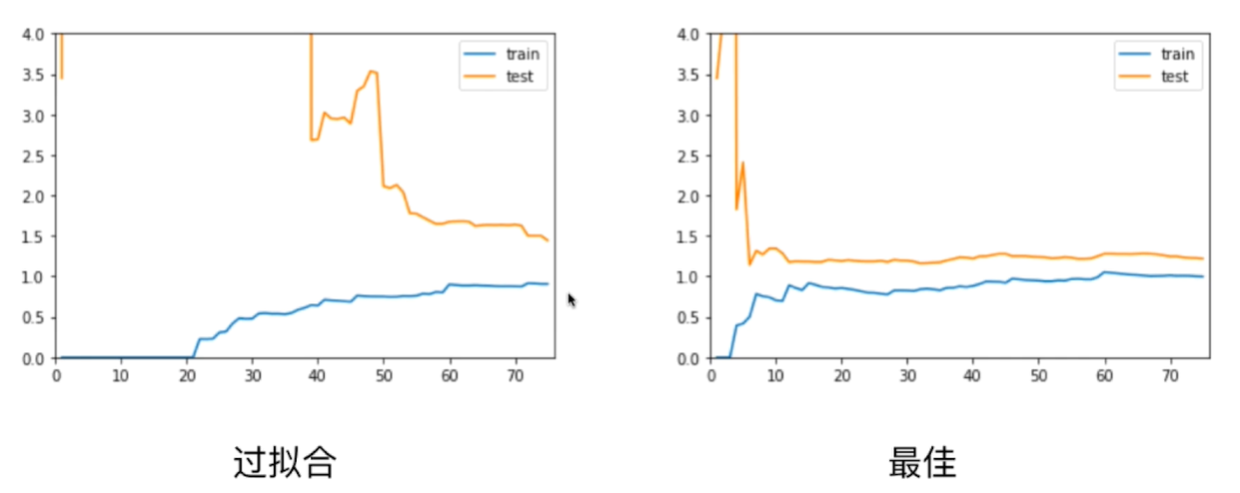
plot_learning_curves_with_algo(X, y, PolynomialRegression(degree=20))
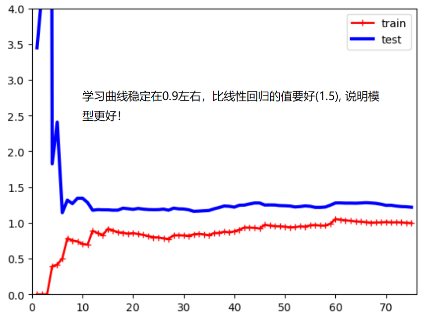
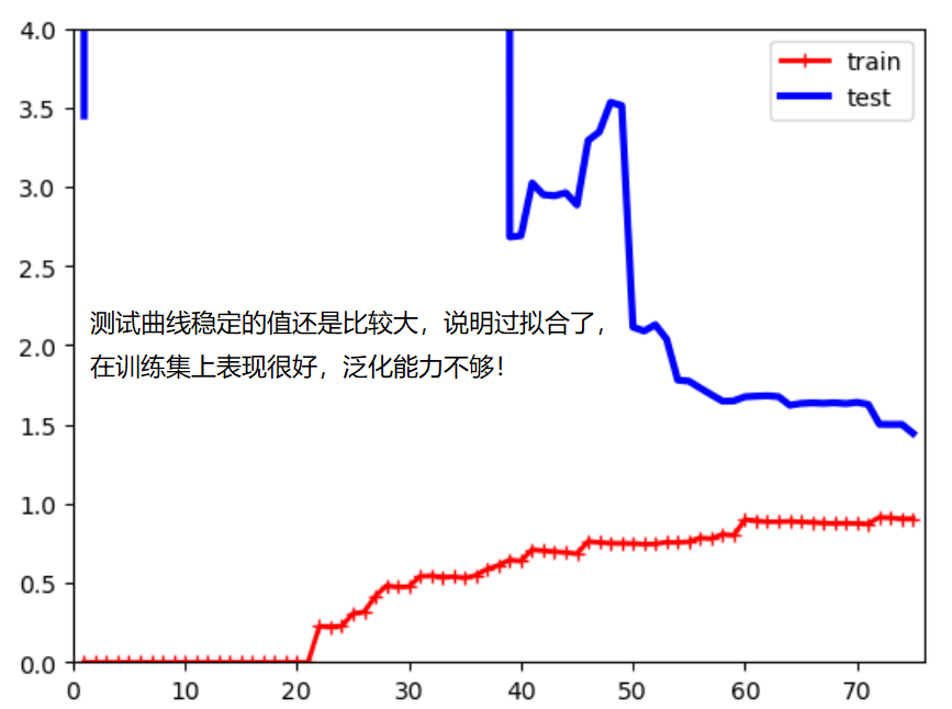
欠拟合的情况下,训练数据集和测试数据集的拟合结果误差都较大!模型不对。
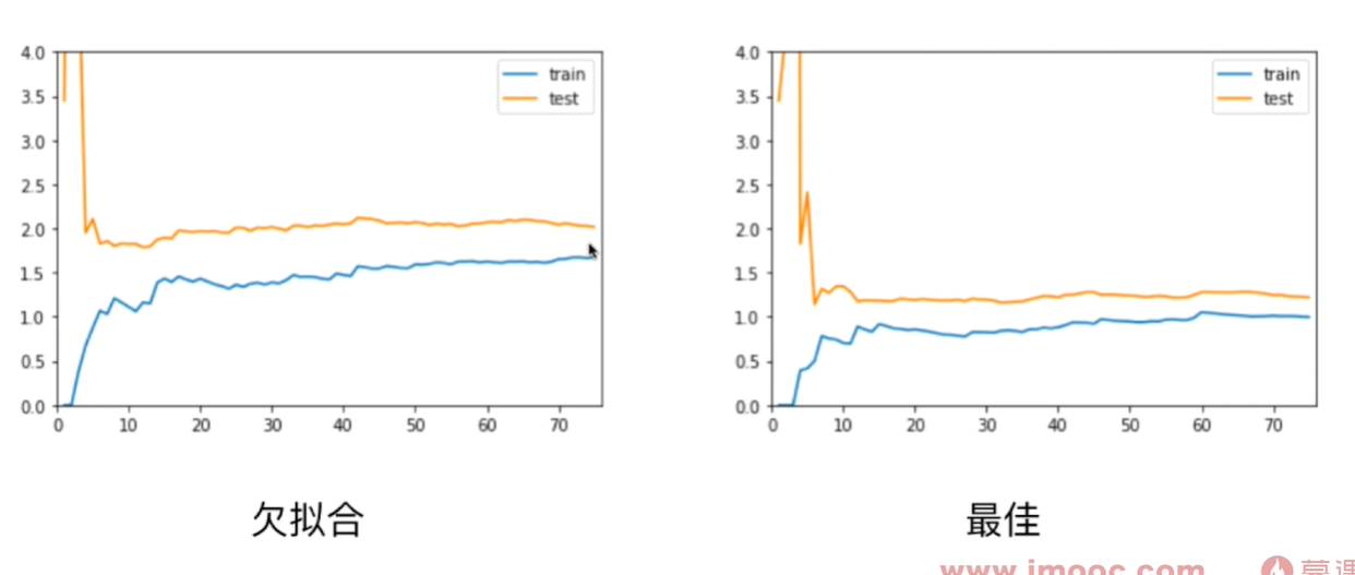
过拟合的情况下,训练数据集的误差和最佳拟合的误差差不多,但是测试数据集的误差很大。测试集的误差和训练集的误差相差较远。 泛化能力不够好!
验证数据集与交叉验证
训练测试数据集分离可能导致过拟合特定的测试数据, 模型围绕着测试数据集打转!针对这个特定测试数据集进行调参。- 过拟合
将数据集分成3部分: 训练数据集,验证数据集(Validation dataset),和测试数据集 原来的测试数据集用验证数据集来代替,参与模型的创建, 调整超参数,而测试数据集只是作为衡量最终模型性能的数据集!
为了避免对特定验证数据集过拟合,引入了交叉验证的方式 - Cross Validation
cross_val_score() 默认情况下将训练数据集分成5分,做交叉验证, 返回5个fold对应的score值.
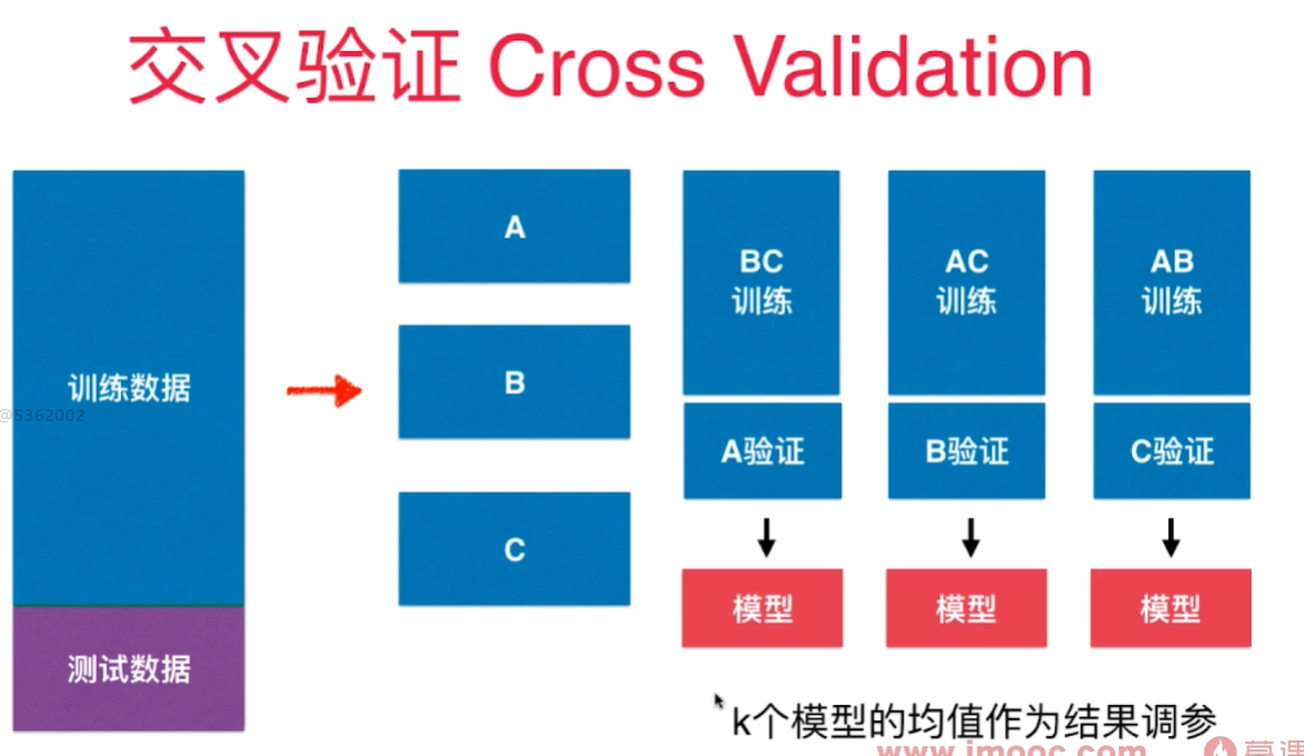
k-folds交叉验证,把数据分成k份,每一份是一个fold。缺点是每次要训练k个模型, 整体性能下降k倍。 极端情况下, 有一个留一法LOO-CV(Leave-one-out cross validation) - 训练集共有m个样本,就将训练数据集分成m份,每次将m-1份样本用于训练, 预测剩下的1个样本。 将这些预测结果做平均,用于衡量模型预测的准确度。 - 完全不受随机的影响, 计算量巨大。 学术论文中可能会采用这个方法用于验证严谨性。
用手写数字集做手动交叉验证:
import numpy as np
from sklearn import datasets
digits = datasets.load_digits()
X = digits.data
y = digits.target

from sklearn.model_selection import train_test_split
X_train, X_test, y_train, y_test = train_test_split(X, y, test_size=0.4, random_state=666)
from sklearn.model_selection import cross_val_score

from sklearn.neighbors import KNeighborsClassifier
best_score, best_k, best_p = 0, 0, 0
for k in range(2, 11):
    for p in range(1, 6):
        knn_clf = KNeighborsClassifier(weights="distance", n_neighbors=k, p=p)
        scores = cross_val_score(knn_clf, X_train, y_train)
        score = np.mean(scores)
        if score > best_score:
            best_score, best_k, best_p = score, k, p
print("Best K = ", best_k)
print("Best P = ", best_p)
print("Best Score = ", best_score)

best_knn_clf = KNeighborsClassifier(weights="distance", n_neighbors=2, p=2)
best_knn_clf.fit(X_train, y_train)
best_knn_clf.score(X_test, y_test)
结果:
Best K =  2
Best P =  2
Best Score =  0.9851507321274763
0.980528511821975
网格搜索:
from sklearn.model_selection import GridSearchCV
param_grid = [
    {
        "weights":['distance'],
        'n_neighbors':[i for i in range(2, 11)],
        'p': [i for i in range(1, 6)]
    }
]

grid_search = GridSearchCV(knn_clf, param_grid, verbose=1)
grid_search.fit(X_train, y_train)
grid_search.best_score_
grid_search.best_params_
best_knn_clf = grid_search.best_estimator_
best_knn_clf.score(X_test, y_test)
结果:
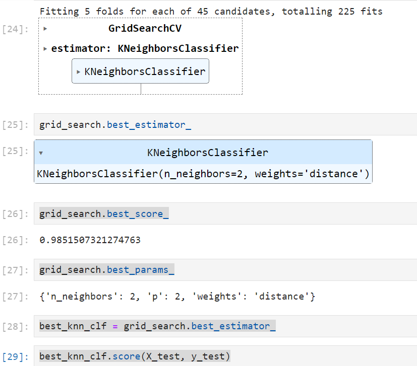
0.980528511821975
偏差方差权衡 - Bias Variance Trade off
偏差 - Bias
高偏差的原因:对问题本身的假设不正确
- 欠拟合 underfitting
- 特征和问题不相关, 比如用名字预测考试成绩
方差 - variance:
数据的一点点扰动就会较大的影响到模型!模型没有完全的学习到问题的实质,而学习到很多噪音。 方差大的通常原因是模型太过复杂,比如用了高阶多项式回归。 - 过拟合会引入方差
不可避免地误差:
数据本身的噪音所致。
模型误差 = 偏差(Bias) + 方差(Variance) + 不可避免地误差
增加模型复杂度会显著提升模型的方差并减少偏差。反过来,降低模型的复杂度则会提升模型的偏差并降低方差 - 权衡
kNN高度的依赖样本数据,决策树也是非参数学习算法,会引入高方差。 参数学习算法通常是高偏差算法。 - 对数据有极强的假设,数据要符合一个数学模型,拟合的目标是求出对应模型的参数。
岭回归(Ridge Regression)
LASSO 回归
让每一个 $\theta$ 尽可能小。 $\alpha$ 用来调整每个 $\theta$ 尽可能小占整个损耗函数的比例
Least abosolute shrinkage and selection operator regression - 有selection功能
selection operator - 选择运算符 - 可以选择特征,theta = 0 的特征完全没有用
LASSO趋向于使一部分theta为0,而不是很小的值,所以可以作为特征选择使用。
弹性网络 Elastic Net
逻辑回归算法 - Logistic Regression
也称为Logit回归
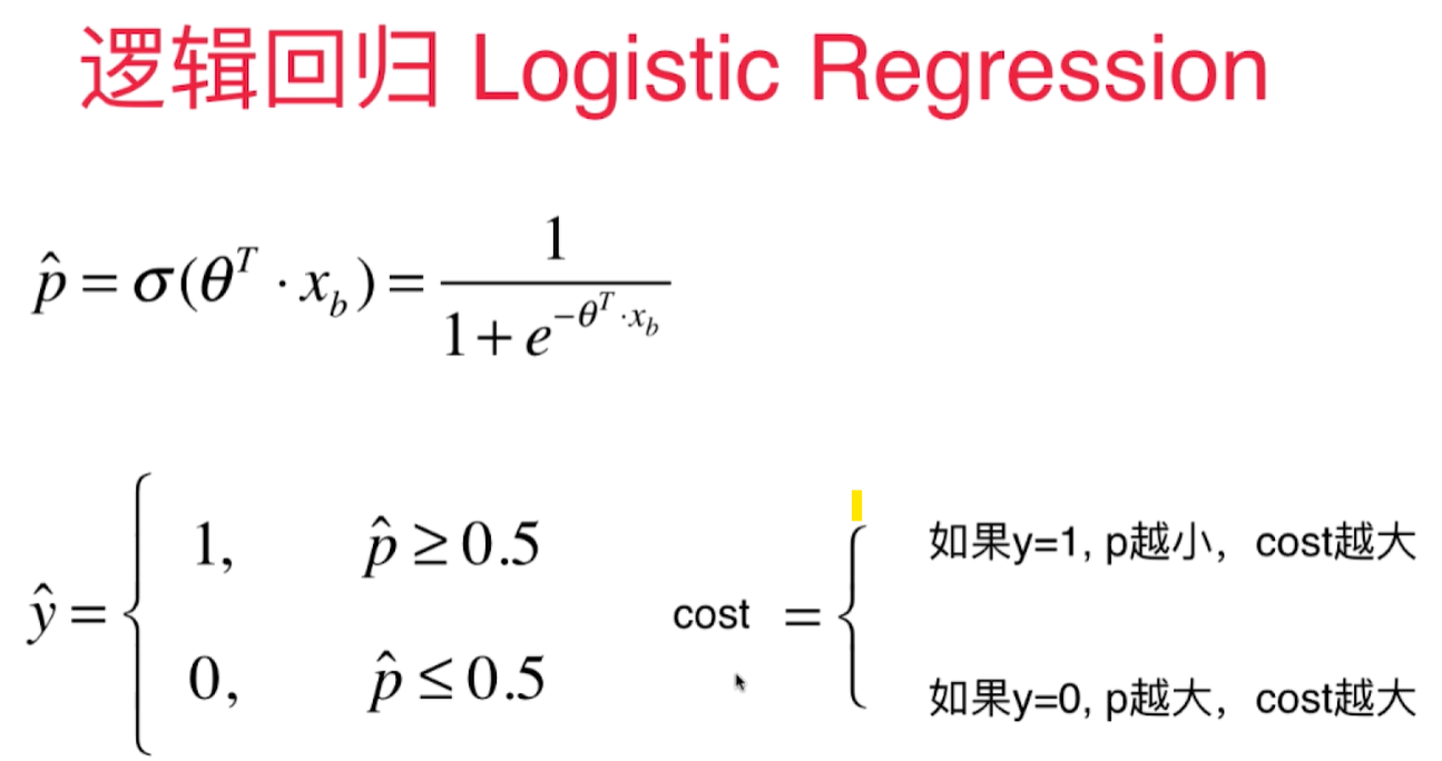
用于解决分类问题,将样本特征和样本发生的概率联系起来. 用于估算一个实例属于某个特定类别的概率。- 是一个二元分类器
首先通过sigmoid函数获得样本对应的属于某个特定值的概率p,然后再根据概率获得 $\hat y$.
$$\hat p = h_{\theta}(x) = \sigma(x^T\theta)$$
$\theta(.)$ 是一个sigmoid函数,输出一个介于0/1之间的数字。
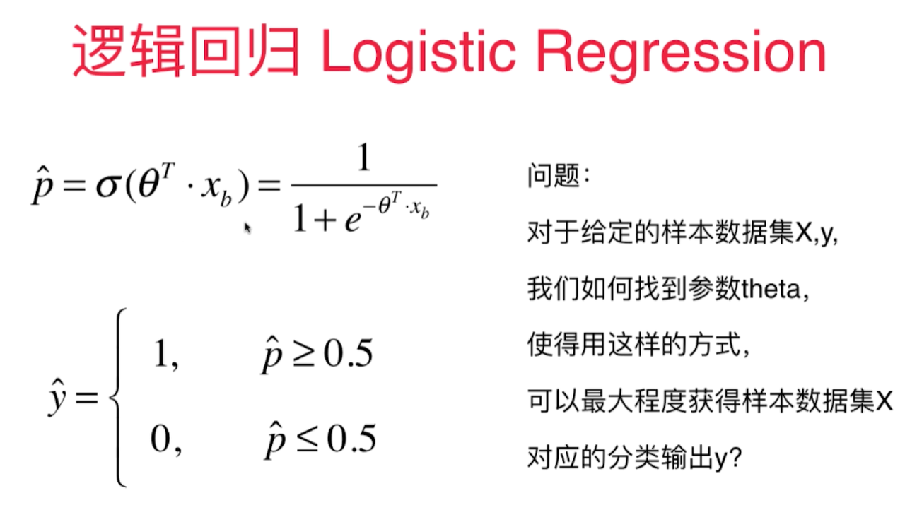
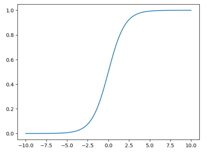
Sigmoid函数:
$$\sigma(t) = \frac{1}{1+e^{-t}}$$
import numpy as np
import  matplotlib.pyplot as plt
def sigmoid(x):
    return 1/(1 + np.exp(-x))
x = np.linspace(-10, 10, 100)
y = sigmoid(x)
plt.plot(x, y)
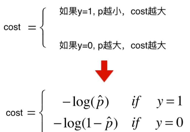
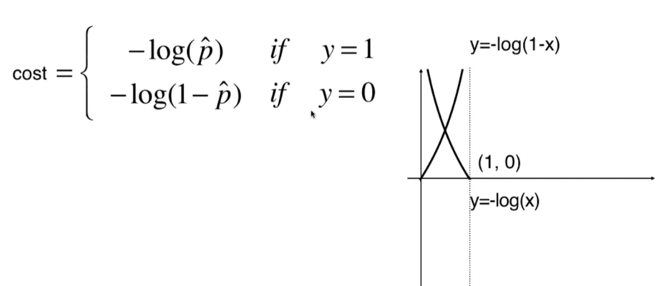
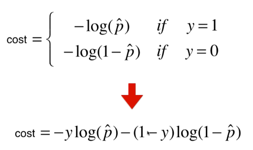
逻辑回归的损失函数
逻辑回归的损失函数不像线性回归那样明显,要从二分类中怎样的行为才是损失最大来考虑:

逻辑回归损失函数的梯度
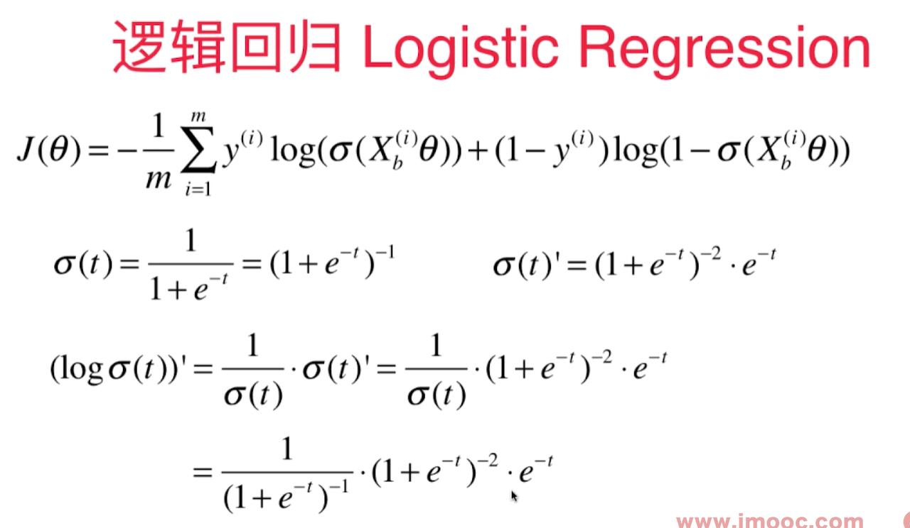
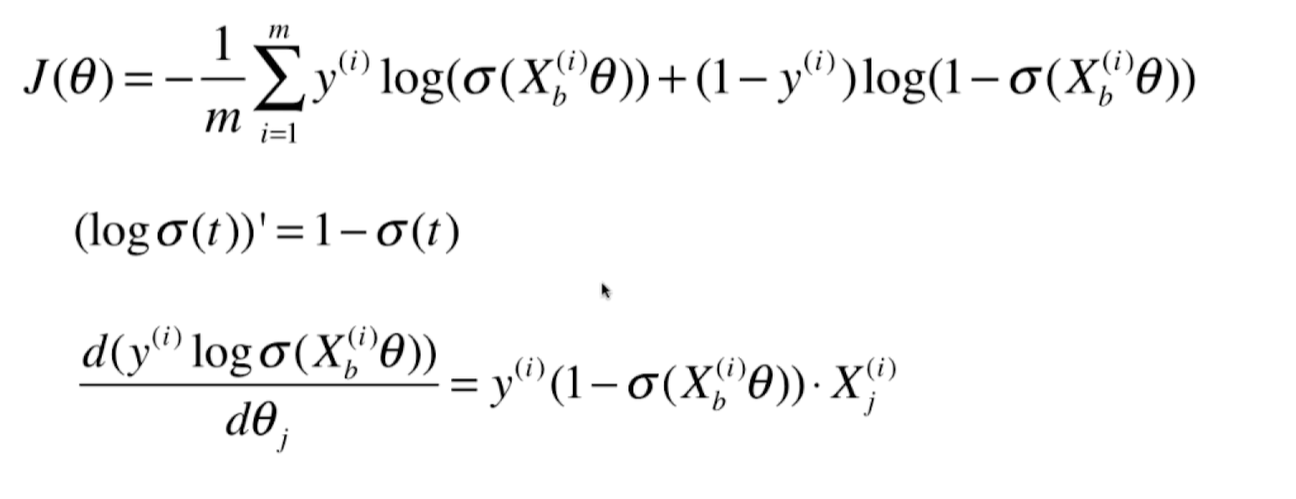
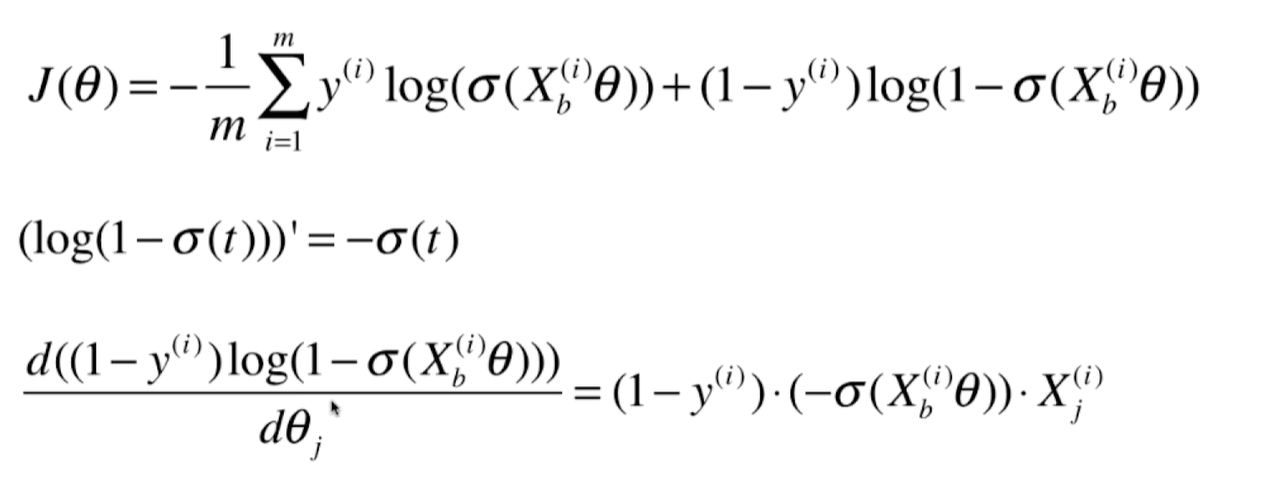
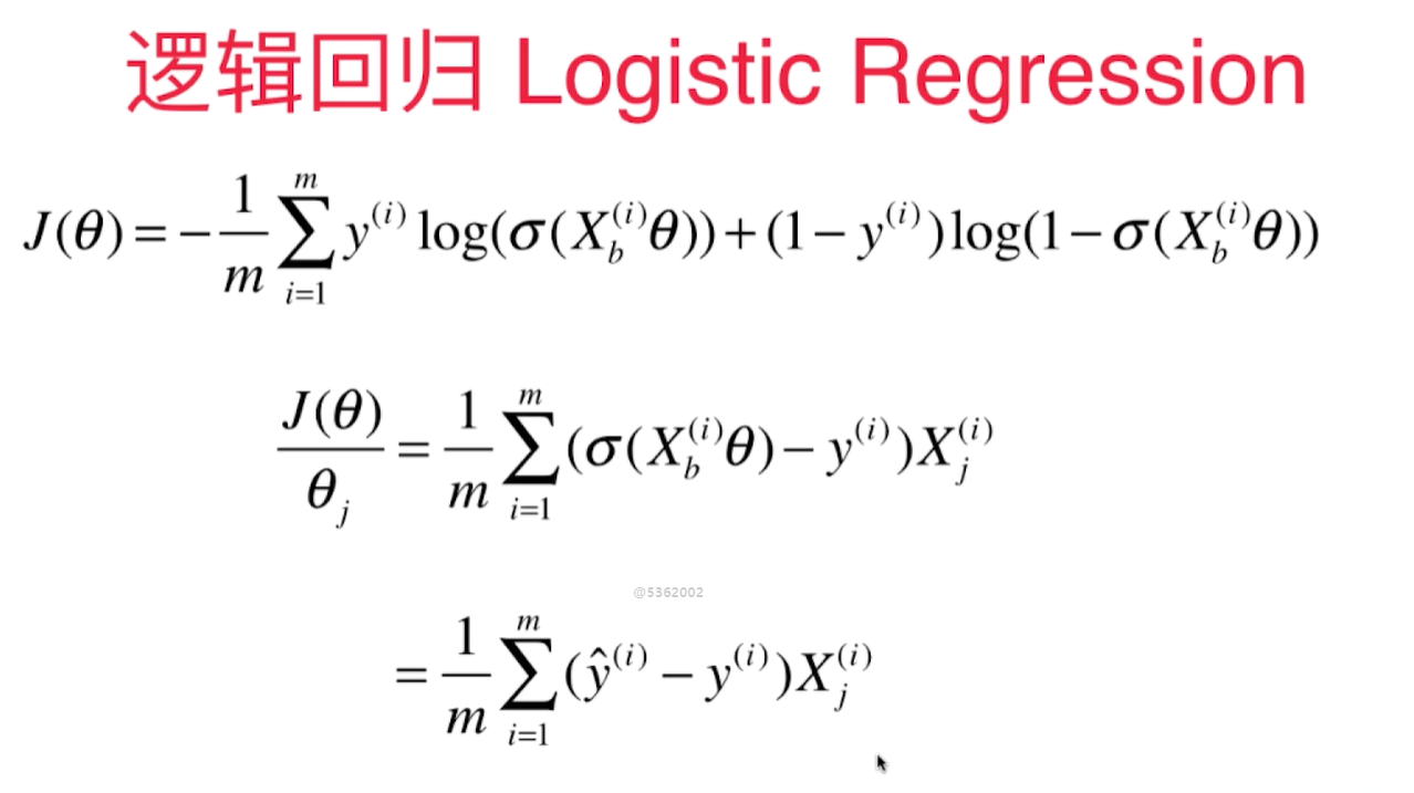
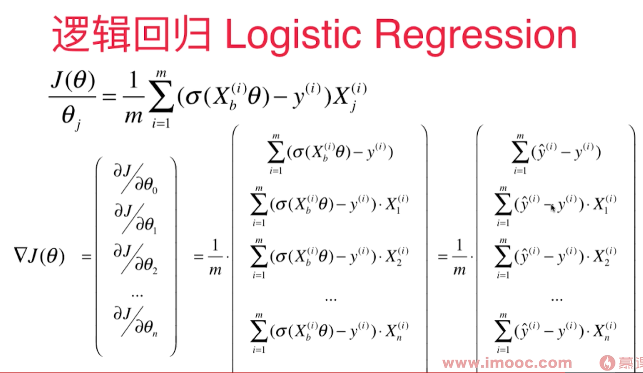 逻辑回归中的梯度公式和线性回归中的梯度公式很像:
2个向量里有共通的部分,每个向量里都有y的预测值( $\hat y$ ) - y 的真值,再乘以 $X_i$ 的第j个维度。然后 $\sum$ 求和,除以m。
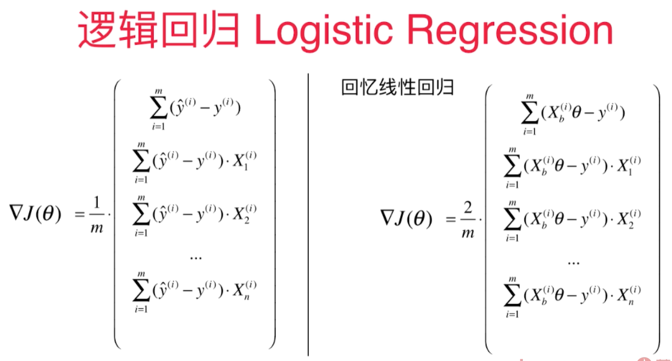 对于线性回归:
$$\hat y = X_b^{i}\theta$$
对于逻辑回归:
$$\hat y = \sigma(X_b^{i}\theta)$$
线性回归多出一个2.
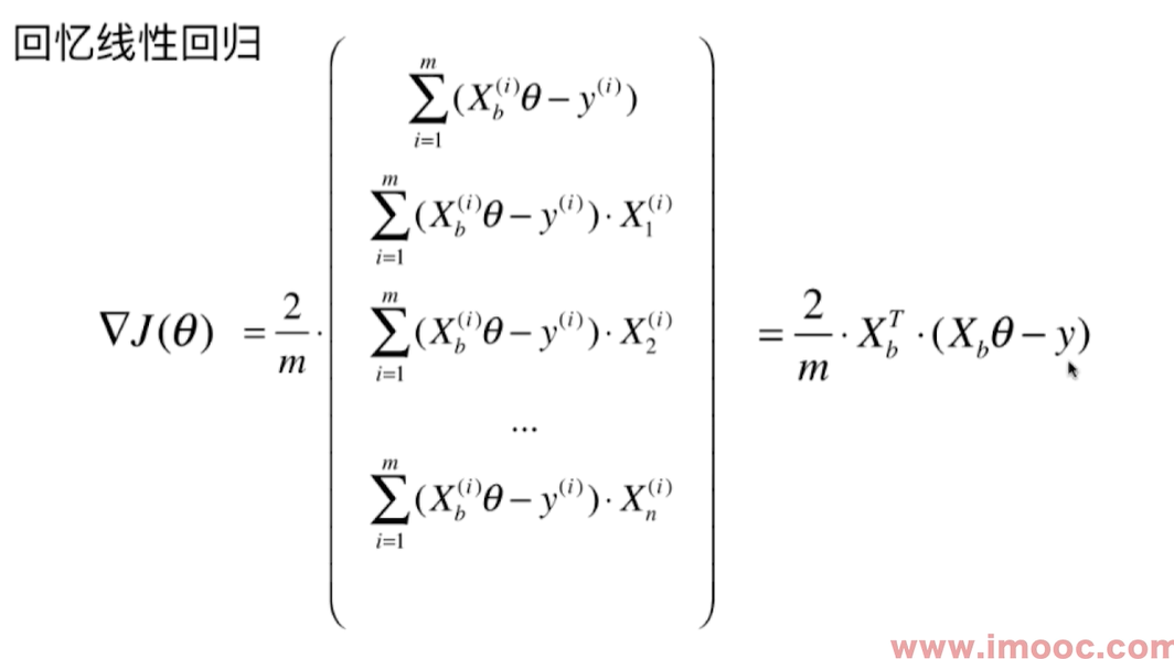
向量化的梯度求解:
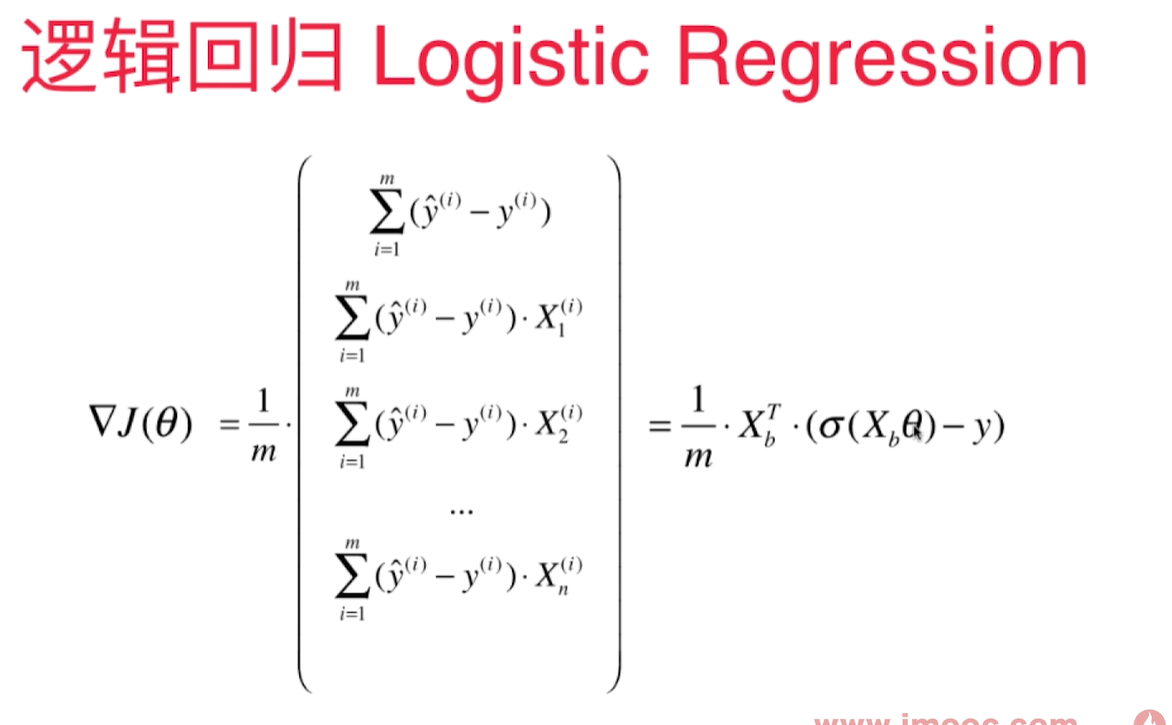
线性回归梯度求解:
实现逻辑回归算法
基于LinearRegression的code实现的LogisticRegression:
import numpy as np
#from .metrics import r2_score


class LogisticRegression:

    def __init__(self):
        """初始化Logistic Regression模型"""
        self.coef_ = None
        self.intercept_ = None
        self._theta = None

    def _sigmoid(self, x):
        return 1 / (1 + np.exp(-x))
    def predict_proba(self, X_predict):
        """给定待预测数据集X_predict,返回表示X_predict的预测概率向量"""
        assert self.intercept_ is not None and self.coef_ is not None, \
            "must fit before predict!"
        assert X_predict.shape[1] == len(self.coef_), \
            "the feature number of X_predict must be equal to X_train"

        X_b = np.hstack([np.ones((len(X_predict), 1)), X_predict])
        return self._sigmoid(X_b.dot(self._theta))
    def predict(self, X_predict):
        """给定待预测数据集X_predict,返回表示X_predict的预测结果向量"""
        assert self.intercept_ is not None and self.coef_ is not None, \
            "must fit before predict!"
        assert X_predict.shape[1] == len(self.coef_), \
            "the feature number of X_predict must be equal to X_train"

        X_b = np.hstack([np.ones((len(X_predict), 1)), X_predict])
        proba = self.predict_proba(X_predict)
        return np.array(proba >= 0.5, dtype = 'int')
    def score(self, X_test, y_test):
        """根据测试数据集 X_test 和 y_test 确定当前模型的准确度"""

        y_predict = self.predict(X_test)
        #return accuracy_score(y_test, y_predict)

    def __repr__(self):
        return "LogisticRegression()"

    def fit(self, X_train, y_train, eta = 0.01, n_iters=1e4):
        assert X_train.shape[0] == y_train.shape[0], "The X_train's size should be equal to the y_train's size"

        def dJ(theta, X_b, y):
           return X_b.T.dot(self._sigmoid(X_b.dot(theta)) - y) / len(y)
        def J(theta, X_b, y):
            try:
                y_hat = self._sigmoid(X_b.dot(theta))
                sum = np.sum(y*np.log(y_hat) + (1 - y)*log(1 - y_hat))
                return -1 * sum/len(y)
            except:
                return float('inf')

        def gradient_descent(X_b, y, initial_theta, eta, n_iters, epsilon=1e-8):
            theta = initial_theta
            i_iter = 0

            while (i_iter < n_iters):
                last_theta = theta
                gradient = dJ(theta, X_b, y)
                theta = theta - eta*gradient
                if np.abs(J(theta, X_b, y) - J(last_theta, X_b, y)) < epsilon:
                    break
                i_iter += 1
            return theta

        X_b = np.hstack((np.ones((len(X_train), 1)), X_train))
        initial_theta = np.zeros(X_b.shape[1])
        self._theta = gradient_descent(X_b, y_train, initial_theta, eta, n_iters)
        self.coef_ = self._theta[1:]
        self.intercept_ = self._theta[0]
        return self
类的成员函数的参数都以 self开始。
iris测试代码:
import numpy as np
import matplotlib.pyplot as plt
import sys
sys.path.append(r'C:\\N-20KEPC0Y7KFA-Data\\junhuawa\\Documents\\00-Play-with-ML-in-Python\\Jupyter')
import playML
from playML.LogisticRegression import LogisticRegression
log_reg = LogisticRegression()
from sklearn import datasets
iris = datasets.load_iris()
X = iris.data
y = iris.target
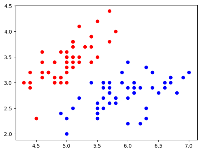
X = X[y<2, :2]#取2个样本特征做可视化
y = y[y < 2] #因为逻辑回归只能做二分类,所以只取前2种数据
plt.scatter(X[y==0, 0], X[y==0, 1], color='r')
plt.scatter(X[y==1, 0], X[y==1, 1], color='b')
from sklearn.model_selection import train_test_split
X_train, X_test, y_train, y_test = train_test_split(X, y)
log_reg.fit(X_train, y_train)
y_predict = log_reg.predict_proba(X_test)
y_hat = log_reg.predict(X_test)
决策边界 - Decision Boundary
逻辑回顾算法也有系数和截距,这些theta的值有什么几何意义呢?
逻辑回归算出每个样本的概率 $\hat p$, $\hat p$ 的值以0.5为界, >= 0.5判定为1, < 0.5 判定为0. 所以0.5对应着决策边界, 0.5意味着 $\theta^T\cdot x_b = 0$, 这个点被称为决策边界。
对于$X$有2个特征的情况:
$$\theta_0 + \theta_1 x_1 + \theta_2 x_2 = 0$$
$$x_2 = \frac {-(\theta_0 + \theta_1 x_1)} {\theta_2}$$
鸢尾花数据集2个特征情况下的决策边界:
import numpy as np
import matplotlib.pyplot as plt
import sys
sys.path.append(r'C:\\N-20KEPC0Y7KFA-Data\\junhuawa\\Documents\\00-Play-with-ML-in-Python\\Jupyter')
import playML
from playML.LogisticRegression import LogisticRegression
log_reg = LogisticRegression()
from sklearn import datasets
iris = datasets.load_iris()
X = iris.data
y = iris.target
X = X[y<2, :2]#因为逻辑回归只能做二分类,所以只取前2种数据
y = y[y < 2]
from sklearn.model_selection import train_test_split
X_train, X_test, y_train, y_test = train_test_split(X, y, random_state=666)
log_reg.fit(X_train, y_train)
theta0 = log_reg.intercept_
theta1 = log_reg._theta[1]
theta2 = log_reg._theta[2]
x2 = (-theta0 - theta1 * X[:, 0])/theta2
plt.scatter(X[y==0, 0], X[y==0, 1], color='r')
plt.scatter(X[y==1, 0], X[y==1, 1], color='b')
plt.plot(X[:, 0], x2)
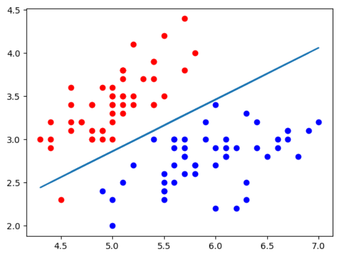
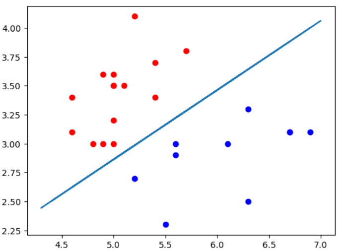
如果只显示测试数据的话,可以看到2种类型的点被边界完美区分,所以测试score = 1.0.
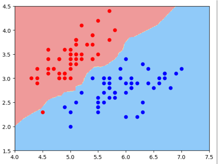
不规则的决策边界绘制方法: kNN 算法也是分类算法,也有决策边界,只是它的决策边界不是一条直线。这种不规则边界可以用下面 plot_decision_boundary()函数来绘制:
def plot_decision_boundary(model, axis):
    x0, x1 = np.meshgrid(
        np.linspace(axis[0], axis[1], int((axis[1] - axis[0])*100)).reshape(-1, 1),
        np.linspace(axis[2], axis[3], int((axis[3] - axis[2])*100)).reshape(-1, 1)
    )
    X_new = np.c_[x0.ravel(), x1.ravel()]

    y_predict = model.predict(X_new)
    zz = y_predict.reshape(x0.shape)

    from matplotlib.colors import ListedColormap
    custom_cmap = ListedColormap(['#EF9A9A', '#FFF59D', '#90CAF9'])
    plt.contourf(x0, x1, zz, cmap=custom_cmap)
对于kNN 分类算法,使用默认n_neighbors时得到的决策边界如下:
from sklearn.neighbors import KNeighborsClassifier
knn_clf = KNeighborsClassifier()
knn_clf.fit(X, y)
plot_decision_boundary(knn_clf, axis=[4, 7.5, 1.5, 4.5])
plt.scatter(X[y==0, 0], X[y==0, 1], color='r')
plt.scatter(X[y==1, 0], X[y==1, 1], color='b')
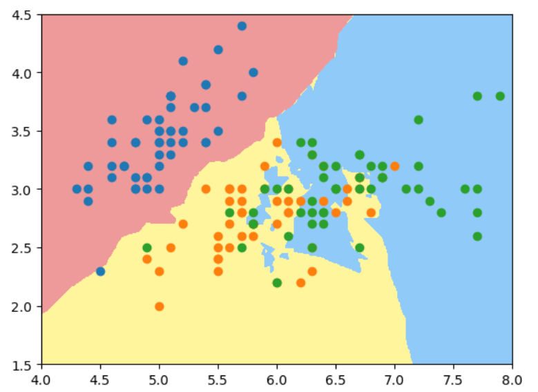
如果用2维特征样本分类3种鸢尾花, 使用默认n_neighbors, 过拟合明显:
X = iris.data[:, :2]
y = iris.target
knn_clf_all = KNeighborsClassifier()
knn_clf_all.fit(X, y)
plot_decision_boundary(knn_clf_all, axis=[4, 8, 1.5, 4.5])
plt.scatter(X[y==0, 0], X[y==0, 1])
plt.scatter(X[y==1, 0], X[y==1, 1])
plt.scatter(X[y==2, 0], X[y==2, 1])
当我们将n_neighbors增大到50时:
knn_clf_50 = KNeighborsClassifier(n_neighbors = 50)
knn_clf_50.fit(X, y)
plot_decision_boundary(knn_clf_50, axis=[4, 8, 1.5, 4.5])
plt.scatter(X[y==0, 0], X[y==0, 1])
plt.scatter(X[y==1, 0], X[y==1, 1])
plt.scatter(X[y==2, 0], X[y==2, 1])
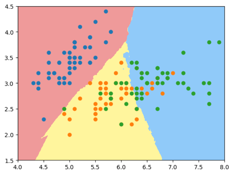
结论: 对于kNN算法,k的值越大,模型越简单,越不容易过拟合。
逻辑回归中使用多项式特征
引入多项式项从而可以得到曲线边界。
$$ x_1^2 + x_2^2 - r^2 = 0$$
将 $x_1^2$ 视为一个特征,$x_2^2$ 视为一个特征,这样就变成了求解一个线性的决策边界。但对于 $x_1$, $x_2$就变成了一个非线性,圆形的决策边界了。
用线性回归转到多项式回归的方法,同理可以让线性逻辑回归转化成多项式逻辑回归。这样就可以对非线性的数据做比较好的分类。 决策边界可以是曲线的形状。
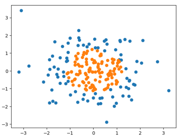
测试数据:
import numpy as np
import matplotlib.pyplot as plt
np.random.seed(666)
X = np.random.normal(0, 1, size = (200, 2))
y = np.array(X[:, 0]**2 + X[:, 1]**2 < 1.5, dtype='int')
plt.scatter(X[y==0, 0], X[y==0, 1])
plt.scatter(X[y==1, 0], X[y==1, 1])
import sys
sys.path.append(r'C:\\N-20KEPC0Y7KFA-Data\\junhuawa\\Documents\\00-Play-with-ML-in-Python\\Jupyter')
import playML
from playML.LogisticRegression import LogisticRegression
from sklearn.pipeline import Pipeline
from sklearn.preprocessing import PolynomialFeatures
from sklearn.preprocessing import StandardScaler
def PolynomialLogisticRegression(degree):
    return Pipeline([
        ('poly', PolynomialFeatures(degree = degree)),
        ('std_scaler', StandardScaler()),
        ('log_reg', LogisticRegression())
    ])
poly_log_reg = PolynomialLogisticRegression(degree = 2)
poly_log_reg.fit(X, y)
plot_decision_boundary(poly_log_reg, [-4, 4, -4, 4])
plt.scatter(X[y==0, 0], X[y==0, 1])
plt.scatter(X[y==1, 0], X[y==1, 1])
plt.title("degree = 2")
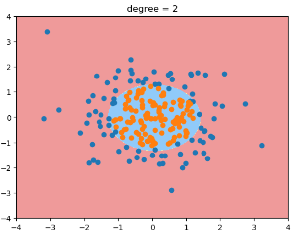
当degree=20时,决策边界变得很奇怪! 过拟合。 - 除了简化模型之外,还可以通过模型正则化来解决过拟合的问题。
逻辑回归中使用正则化
多项式回归中引入L2 或 L1正则项:
$$J(\theta) + \alpha L_2 $$
$$J(\theta) + \alpha L_1 $$
引入一个新的正则化超参数: $C$
$$C\cdot J(\theta) + L1$$
$$C\cdot J(\theta) + L2$$
C越大(1000, 10000),则 $J(\theta)$ 的影响力越小. C越小,比如0.1, 0.01, 则L1/L2正则项更加重要, 因为L1/L2是$\theta$项, 也即 $\theta$ 项尽可能小。
正则项L1, L2, 正则项 $C$ 可以看成是 $L1$, $L2$ 前面的 $\alpha$ 的倒数。 在逻辑回归和SVM算法中,sklearn中的正则化更偏好用 $C$, 而不是用$\alpha$ .这样可以保证必须做正则化. 也提醒我们对于一些逻辑复杂的算法,都应该加上正则化。
sklearn中的LogisticRegression自带了正则化功能,有多个超参数可以配置:
- penalty, 'l2' in default
- C, 1.0 in default
- solver, lbfgs in default
- ......
决策边界为抛物线的测试代码:
import numpy as np
import matplotlib.pyplot as plt
np.random.seed(666)
X = np.random.normal(0, 1, size=(200, 2))# 有200个样本,每个样本2个特征
y = np.array(X[:, 0]**2 + X[:, 1] < 1.5, dtype='int')
for _ in range(20): # 加入20个噪音
    y[np.random.randint(200)] = 1
用线性逻辑回归拟合一个决策边界为抛物线的样本的结果:
from sklearn.model_selection import train_test_split
X_train, X_test, y_train, y_test = train_test_split(X, y, random_state=666)
from sklearn.linear_model import LogisticRegression
log_reg = LogisticRegression()
log_reg.fit(X_train, y_train)
plot_decision_boundary(log_reg, axis=[-4, 4, -4, 4])
plt.scatter(X[y==0, 0], X[y==0, 1])
plt.scatter(X[y==1, 0], X[y==1, 1])
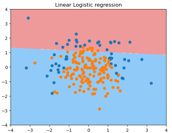
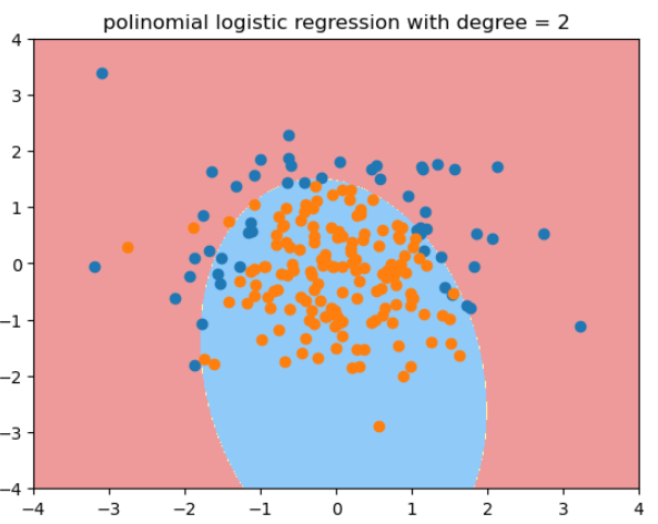
用度为2的多项式逻辑回归拟合的结果:
from sklearn.pipeline import Pipeline
from sklearn.preprocessing import PolynomialFeatures
from sklearn.preprocessing import StandardScaler
def PolynomialLogisticRegression(degree):
    return Pipeline([
        ('poly', PolynomialFeatures(degree = degree)),
        ('std_scaler', StandardScaler()),
        ('log_reg', LogisticRegression())
    ])
poly_log_reg = PolynomialLogisticRegression(degree=2)
poly_log_reg.fit(X_train, y_train)
plot_decision_boundary(poly_log_reg, axis=[-4, 4, -4, 4])
plt.scatter(X[y==0, 0], X[y==0, 1])
plt.scatter(X[y==1, 0], X[y==1, 1])
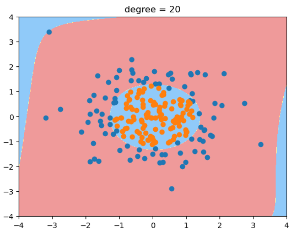
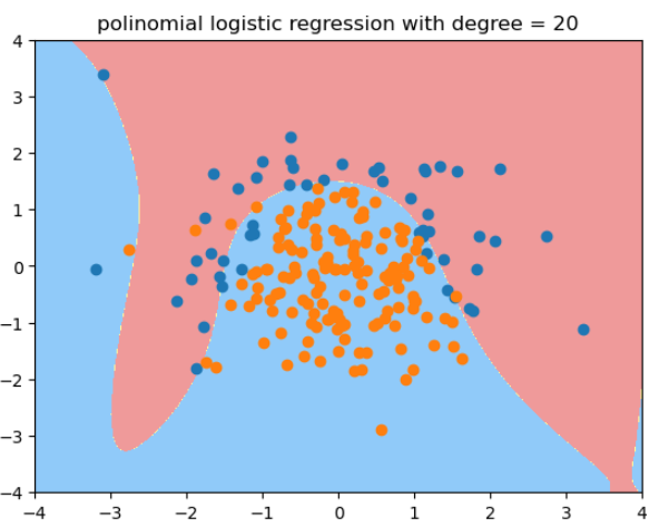
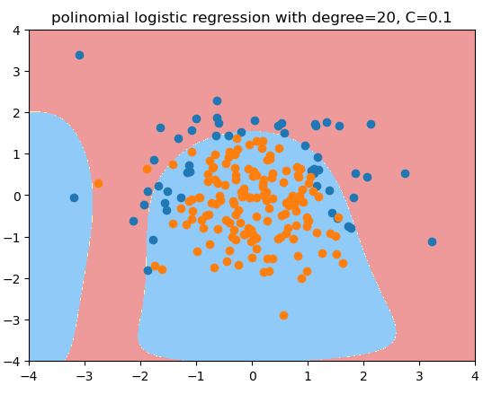
用度为20的多项式逻辑回归拟合的结果: -
用度为20, C=0.1的多项式逻辑回归拟合的结果, 更倾向于degree=2的情况:
def PolynomialLogisticRegression(degree, C, penalty = 'l2', solver='liblinear'):
    return Pipeline([
        ('poly', PolynomialFeatures(degree = degree)),
        ('std_scaler', StandardScaler()),
        ('log_reg', LogisticRegression(C = C, penalty = penalty, solver=solver))
    ])
poly_log_regc = PolynomialLogisticRegression(degree=20, C=0.1, solver='liblinear')# 正则化权重大,分类损失函数权重小,
poly_log_regc.fit(X_train, y_train)
poly_log_regc.score(X_train, y_train)
poly_log_regc.score(X_test, y_test)
plot_decision_boundary(poly_log_regc, axis=[-4, 4, -4, 4])
plt.scatter(X[y==0, 0], X[y==0, 1])
plt.scatter(X[y==1, 0], X[y==1, 1])
plt.title("polinomial logistic regression with degree=20, C=0.1")
用度为20, C=0.1, penalty='l1'的多项式逻辑回归拟合的结果 - L1正则项可以减少很多多项式项,使其系数为0,逼近期望的结果 - 原始数据的形状
def PolynomialLogisticRegression(degree, C, penalty = 'l2', solver='liblinear'):
    return Pipeline([
        ('poly', PolynomialFeatures(degree = degree)),
        ('std_scaler', StandardScaler()),
        ('log_reg', LogisticRegression(C = C, penalty = penalty, solver=solver))
    ])
poly_log_regc = PolynomialLogisticRegression(degree=20, C=0.1, penalty = 'l1', solver='liblinear')# 正则化权重大,分类损失函数权重小,
poly_log_regc.fit(X_train, y_train)
poly_log_regc.score(X_train, y_train)
poly_log_regc.score(X_test, y_test)
plot_decision_boundary(poly_log_regc, axis=[-4, 4, -4, 4])
plt.scatter(X[y==0, 0], X[y==0, 1])
plt.scatter(X[y==1, 0], X[y==1, 1])
plt.title("polinomial logistic regression with degree=20, C=0.1, penalty=l1")
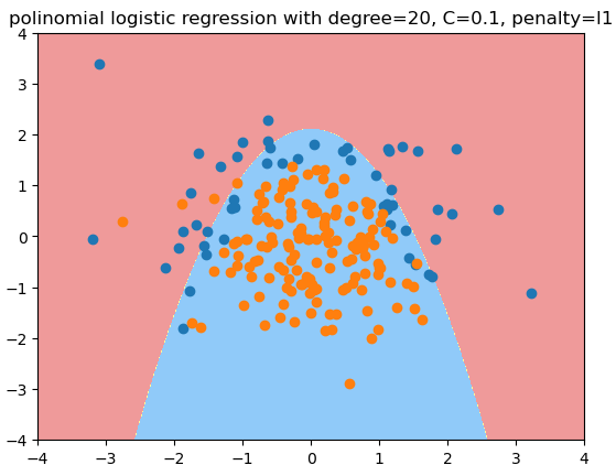
真实环境中,我们不知道哪个degree/C/penalty是最佳的超参数,只能通过网格搜索来获得。
OvR 与 OvO - 逻辑回归解决多分类问题
所有的二分类算法都可以通过以下的方法改造成多分类算法:
-
OvR (One vs Rest) 也叫 (One vs All) 每次只做二分类,区分这个新来的样本点在一个类别和其他的类别中的预测值,然后对其他类别也做这样的分类,得到在每个分类上的预测值,取最大的值对应的类别为这个新来样本点的类别。
n个类别就要n个分类, 处理一个分类要T, 则要N*T的复杂度 -
OvO (One vs One) 每次只挑出2个类别进行二分类, 如果总共有4个类别,则可以形成 $C_4^2 = 6$ 对这样的分类。 复杂度: $C_n^2 * T$. 因为每次都只用2个类别比较,没有混淆其他类别的信息,所有分类会更加准确。
sklearn 中的Logistic Regression默认支持多分类,用超参数为 multi_class = 'ovr' or 'ovo'
我这个版本sklearn默认使用 multiclass='ovo', solver='newton-cg' 方式, 既ovo mode. 可以通过使用multiclass='ovr', solver='liblinear'改成ovr mode.
鸢尾花测试数据用2维样本特征做3分类:
import numpy as np
import matplotlib.pyplot as plt
from sklearn.linear_model import LogisticRegression
from sklearn import datasets
iris = datasets.load_iris()
X = iris.data
y = iris.target
X = X[:, :2]#为了可视化,这里只取iris里的前2个维度作为特征进行fit
y = y[:] #分类3中鸢尾花,不再是二分类问题,而是多分类问题了

from sklearn.model_selection import train_test_split
X_train, X_test, y_train, y_test = train_test_split(X, y, random_state=666)

def plot_decision_boundary(model, axis):
    x0, x1 = np.meshgrid(
        np.linspace(axis[0], axis[1], int((axis[1] - axis[0])*100)).reshape(-1, 1),
        np.linspace(axis[2], axis[3], int((axis[3] - axis[2])*100)).reshape(-1, 1)
    )
    X_new = np.c_[x0.ravel(), x1.ravel()]

    y_predict = model.predict(X_new)
    zz = y_predict.reshape(x0.shape)

    from matplotlib.colors import ListedColormap
    custom_cmap = ListedColormap(['#EF9A9A', '#FFF59D', '#90CAF9'])
    plt.contourf(x0, x1, zz, cmap=custom_cmap)
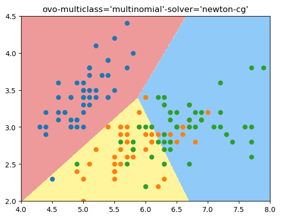
ovo 多分类模式:
log_reg = LogisticRegression()
log_reg.fit(X_train, y_train)
log_reg.score(X_test, y_test)
plot_decision_boundary(log_reg, [4, 8, 2, 4.5])
plt.scatter(X[y==0, 0], X[y==0, 1])
plt.scatter(X[y==1, 0], X[y==1, 1])
plt.scatter(X[y==2, 0], X[y==2, 1])
结果:
score: 0.7894736842105263
ovr模式:
log_reg1 = LogisticRegression(multi_class='ovr', solver='liblinear') # 这个方式是ovr的方式
log_reg1.fit(X_train, y_train)
log_reg1.score(X_test, y_test)
plot_decision_boundary(log_reg1, [4, 8, 2, 4.5])
plt.scatter(X[y==0, 0], X[y==0, 1])
plt.scatter(X[y==1, 0], X[y==1, 1])
plt.scatter(X[y==2, 0], X[y==2, 1])
plt.title("ovr-multiclass='ovr'-solver='liblinear'")
结果:
score: 0.6578947368421053
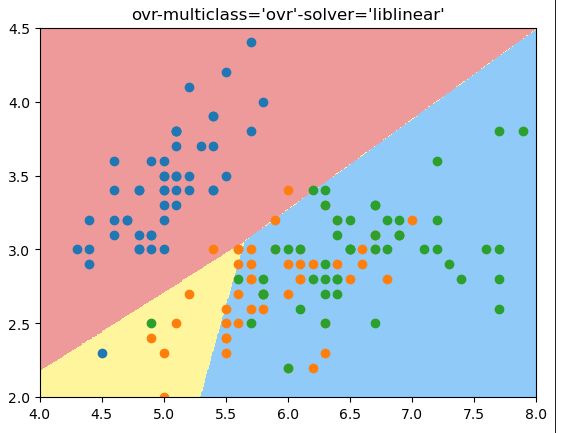
结论:可以看出来,ovr得到的准确度没有ovo好,从决策边界看,ovo的决策边界也更合理
OvO and OvR 分类器
sklearn提供了OvO and OvR 分类器,任何一个二分类算法都可以用这2个分类器实现多分类功能。
from sklearn.multiclass import OneVsRestClassifier
X = iris.data
y = iris.target
X_train, X_test, y_train, y_test = train_test_split(X, y, random_state=666)
log_reg1 = LogisticRegression(multi_class='ovr', solver='liblinear')
ovr = OneVsRestClassifier(log_reg1)
ovr.fit(X_train, y_train)
ovr.score(X_test, y_test)
score: 0.9473684210526315
from sklearn.multiclass import OneVsOneClassifier
ovo = OneVsOneClassifier(log_reg)
ovo.fit(X_train, y_train)
ovo.score(X_test, y_test)
score: 1.0
准确度陷阱和混淆矩阵(confusion matrix)
对于有偏的数据(skewed data)二分类时使用的度量指标:
对于二分类问题,很难用准确度来度量算法的好坏,比如有一个算法,用10000个人的体检样本来预测得癌症的准确率是99.99%, 如果在这个算法中把所有的人都默认预测为不会得癌症(0), 也完全符合前面99.99%的要求,因为样本中本身得癌症的样本就很少。 所以用准确度 (accuracy_score) 无法区分这个算法性能到底是怎么样的。 所以引入了混淆矩阵, 精准度, 召回率和 ROC曲线等来度量二分法性能的优略.
混淆矩阵
矩阵每一行代表样本的真实结果,每一列代表样本的预测结果,每一行列都是从 0(预测为阴 Negative) 开始, 再是 1(预测为阳 positive):
在矩阵中,每一个格子用两个字符来表示其含义,第二个字符表示预测的结果,第一个字符表示预测结果和真实结果相比是真还是假。
| 真实值 | 预测值 | 0 | 1 |
|---|---|---|
| 0 | TN(True Negative) | FP (False Positive) |
| 1 | FN(False Negative) | TP (True Positive) |
精准率 - Precision score
$$ Precision\ score = \frac {TP} {TP + FP} $$
召回率 - Recall score
$$ Recall\ score = \frac {TP} {TP + FN} $$
$F_1\ Score$ - Balanced F score
精准率和召回率的调和平均值,如果一个值特别低,得到的值也将特别低, 只有 2 者都高的时候才会特别高.
$$ \frac 1 {F_1} = \frac 1 2 (\frac 1 {precision} + \frac 1 {recall}) $$
$$ F_1\ Score = \frac {2} {\frac 1 {精度} + \frac 1 {召回率} } = \frac {TP} {TP + \frac {FN + FP} 2} $$
不同的应用场景,关注的二分类指标是不一样的,比如股票预测注重精准率,不关注召回率。 医疗领域的病人诊断中我们注重召回率,不想漏掉任何患病的人群,但是精准率就不那么重要了。
同时关注精准率和召回率 $F_1\ score$
sklearn 中的实现
from sklearn.metrics import precision_score
from sklearn.metrics import recall_score
from sklearn.metrics import confusion_metrix
from sklearn.metrics import f1_score
confusion_metrix(y_test, y_predict)
array([[403,   2],
       [  9,  36]], dtype=int64)
精准率和召回率的平衡
下图圆圈代表真值为0, 五角星代表真值为1,score(既横轴)代表每个样本点的score, 0代表默认的决策边界, 既 $ \theta^T \cdot x_b = 0$.
当决策边界往右移动时, 既 $\theta^T\cdot x_b=Val, val>0$, 精准率提高,召回率下降。
当决策边界往左移动时, 既 $\theta^T\cdot x_b=Val, val<0$, 召回率提高,精准率下降。
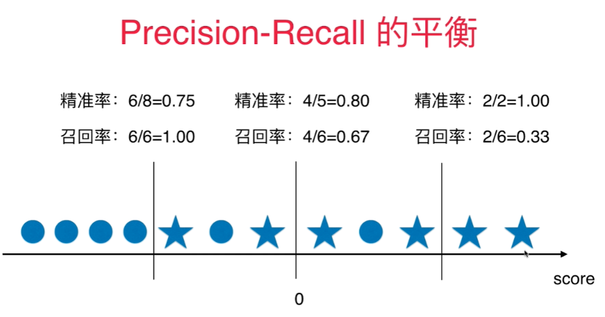
精准率和召回率的平衡通过调整分类为1的阈值来完成, 像逻辑回归分类算法通过计算出一个score值,通过score值是否> < 0来具体分类的算法中,sklearn自带一个函数: decision_function(). 做决策的函数。
将X_test传入得到一维向量,其中包含每个样本对应的score值。
sklearn.metrics包含混淆矩阵生成函数,求精准度, 召回率, 和 f1 score 的函数。 不包含修改决策边界阀值的函数,如果要修改,只能通过 decision_function() 间接修改。
测试数据:
import numpy as np
import matplotlib.pyplot as plt
from sklearn.datasets import load_digits
X = load_digits().data
y = load_digits().target
y = np.array( y == 9, dtype='int')
from sklearn.linear_model import LogisticRegression
log_reg = LogisticRegression(solver = 'liblinear')
from sklearn.model_selection import train_test_split
X_train, X_test, y_train, y_test = train_test_split(X, y, random_state = 666)
log_reg.fit(X_train, y_train)
y_predict = log_reg.predict(X_test)
log_reg.score(X_test, y_test)
求解混淆矩阵:
from sklearn.metrics import confusion_matrix
confusion_matrix(y_test, y_predict)
array([[403,   2],
       [  9,  36]], dtype=int64)
求解精准度, 召回率, 和f1 score:
from sklearn.metrics import precision_score
from sklearn.metrics import recall_score
from sklearn.metrics import f1_score
precision_score(y_test, y_predict)
recall_score(y_test, y_predict)
0.9473684210526315
0.8
通过调整决策边界的阀值(threshold), 可以调整精准度和召回率:
把 $>=5$ 设为决策边界的阀值:
scores = log_reg.decision_function(X_test)
y_5 = np.array(scores>=5)
confusion_matrix(y_test, y_5)
precision_score(y_test, y_5)
recall_score(y_test, y_5)
结果:
array([[404,   1],
       [ 21,  24]], dtype=int64)
0.96
0.5333333333333333
把 $>=-5$ 设为决策边界的阀值: 结果:
array([[390,  15],
       [  5,  40]], dtype=int64)
0.7272727272727273
0.8888888888888888
精准率-召回率曲线
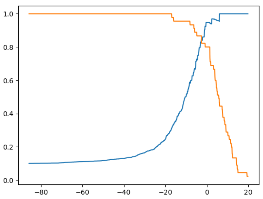
我们可以通过遍历threshold值来计算出各个threshold值对应的precision/recall 值,然后画出这两条曲线:
import numpy as np
import matplotlib.pyplot as plt
from sklearn.datasets import load_digits
X = load_digits().data
y = load_digits().target
y = np.array( y == 9, dtype='int')
from sklearn.linear_model import LogisticRegression
log_reg = LogisticRegression(solver = 'liblinear')
from sklearn.model_selection import train_test_split
X_train, X_test, y_train, y_test = train_test_split(X, y, random_state = 666)
log_reg.fit(X_train, y_train)
y_predict = log_reg.predict(X_test)
绘制精准率和召回率曲线:
from sklearn.metrics import precision_score
from sklearn.metrics import recall_score
decision_scores = log_reg.decision_function(X_test)
from sklearn.metrics import recall_score
thresholds = np.arange(np.min(decision_scores), np.max(decision_scores), 0.1)
precisions = []
recalls = []
for threshold in thresholds:
    y_predict = np.array(decision_scores >= threshold, dtype='int')
    precisions.append(precision_score(y_test, y_predict))
    recalls.append(recall_score(y_test, y_predict))

plt.plot(thresholds, precisions[:-1])
plt.plot(thresholds, recalls[:-1])
也可以用precision和recall值,画出precision-recall曲线,从该曲线里可以看到随着precision值增大,recall值逐渐下降。存在一个零界点,从这个点开始,曲线急剧下降,这个点就是最好的平衡点。
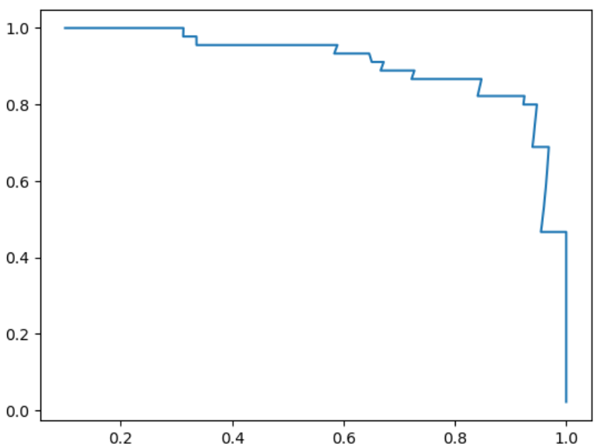
sklearn.metrics也提供了 precision_recall 曲线绘制函数 precision_recall_curve():
from sklearn.metrics import precision_recall_curve
precisions, recalls, thresholds = precision_recall_curve(y_test, decision_scores)
plt.plot(thresholds, precisions[:-1])
plt.plot(thresholds, recalls[:-1])
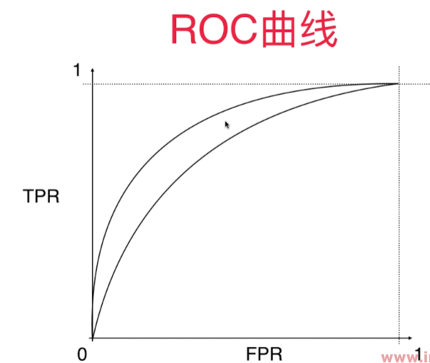
ROC曲线 - Receiver Operation Characteristic Curve
统计学上的概念,用于描述 TPR 和 FPR 之间的关系。
TPR (真正率) = Recall score = $\frac {TP} {TP + FN}$ = 召回率
预测值为1, 并且预测对了的数量占真实值为1的样本比率。
$$ TPR = Recall\ score$$
FPR (False Positive Rate 假阳性率) = $FPR=\frac{FP}{TN+FP}$
预测值为1, 但是预测错了的样本和真实值为0的样本的比率。 - 犯了false positive的错误 - 预测错的正样本 占 全体正样本 的比例,也叫误识别率、虚警率。
TPR 和FPR呈现相一致的趋势,当决策阈值逐渐降低时,TPR和FPR的值逐渐增大。
在playML中实现TPR和FPR:
def TPR(y_true, y_predict):
    return Recall_Score(y_true, y_predict)

def FPR(y_true, y_predict):
    fp = FP(y_true, y_predict)
    tn = TN(y_true, y_predict)
    try:
        return fp/(fp + tn)
    except:
        return 0.0
在notebook里调用:
import numpy as np
import matplotlib.pyplot as plt
import sys
sys.path.append(r'C:\\N-20KEPC0Y7KFA-Data\\junhuawa\\Documents\\00-Play-with-ML-in-Python\\Jupyter')
from playML.metrics import TPR
from playML.metrics import FPR

from sklearn.datasets import load_digits
X = load_digits().data
y = load_digits().target
y = np.array( y == 9, dtype='int')
from sklearn.linear_model import LogisticRegression
log_reg = LogisticRegression(solver = 'liblinear')
from sklearn.model_selection import train_test_split
X_train, X_test, y_train, y_test = train_test_split(X, y, random_state = 666)
log_reg.fit(X_train, y_train)
#y_predict = log_reg.predict(X_test)
decision_scores = log_reg.decision_function(X_test)

thresholds = np.arange(np.min(decision_scores), np.max(decision_scores), 0.1)
tprs = []
fprs = []
for threshold in thresholds:
    y_predict = np.array(decision_scores >= threshold, dtype='int')
    fprs.append(FPR(y_test, y_predict))
    tprs.append(TPR(y_test, y_predict))

plt.plot(fprs, tprs)
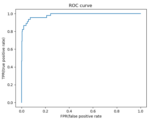
Sklearn 中的ROC曲线和AUC
from sklearn.metrics import roc_curve
fpr, tpr, thresholds = roc_curve(y_test, decision_scores)
plt.plot(fpr, tpr)
plt.title("ROC curve ")
plt.xlabel("FPR(false positive rate")
plt.ylabel("TPR(true positive rate)")
from sklearn.metrics import roc_auc_score# 求ROC曲线下的面积
roc_auc_score(y_test, decision_scores)
0.9830452674897119
sklearn.metrics.roc_auc_score - 用于求取ROC曲线下的面积, area under curve.
这个面积越大,这个算法越好。最大值为1.
这个指标对于有偏数据不敏感,不像precision score和recall score那么敏感。 所以, 对于有偏数据,用precision score和recall score 看其性能是非常有必要的。
而ROC/AUC曲线主要用于比较两个模型性能的优劣。 - 要选取AUC面积更大的模型。
多分类问题中的混淆矩阵
sklearn.metrics里的confusion_matrix() 可以直接用于多分类标签场合。 测试代码:
import numpy as np
import matplotlib.pyplot as plt
from sklearn.datasets import load_digits
X = load_digits().data
y = load_digits().target

from sklearn.linear_model import LogisticRegression
log_reg = LogisticRegression(solver = 'liblinear')
from sklearn.model_selection import train_test_split
X_train, X_test, y_train, y_test = train_test_split(X, y, test_size=0.8)
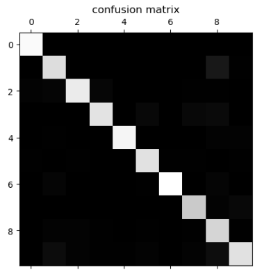
用matplotlib的matshow() 函数可以查看混淆矩阵的图像:
log_reg.fit(X_train, y_train)
log_reg.score(X_test, y_test)
y_predict = log_reg.predict(X_test)
from sklearn.metrics import confusion_matrix
cfm = confusion_matrix(y_test, y_predict)
plt.matshow(cfm, cmap=plt.cm.gray)
array([[146,   0,   0,   0,   0,   0,   0,   0,   0,   0],
       [  0, 129,   0,   0,   0,   0,   0,   0,  14,   1],
       [  2,   3, 137,   4,   0,   0,   0,   1,   1,   0],
       [  0,   0,   0, 133,   0,   5,   0,   5,   6,   0],
       [  0,   1,   0,   0, 143,   0,   0,   0,   2,   2],
       [  1,   0,   1,   0,   0, 131,   1,   1,   0,   1],
       [  0,   3,   0,   0,   0,   1, 149,   0,   3,   0],
       [  0,   0,   0,   0,   0,   0,   0, 118,   2,   5],
       [  0,   2,   2,   1,   0,   1,   0,   1, 124,   1],
       [  0,   7,   2,   1,   1,   2,   0,   2,   8, 131]], dtype=int64)
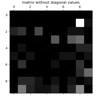
为了把焦点放在错误上,应该把对角线上的值抹去,然后每一个统计值除以总的样本数得到错误率:
cfm = confusion_matrix(y_test, y_predict)
row_sums = cfm.sum(axis=1, keepdims=True)
norm_cfm = cfm/row_sums
np.fill_diagonal(norm_cfm, 0)
plt.matshow(norm_cfm, cmap=plt.cm.gray)
precision_score再添加一个参数就可以支持多分类问题。
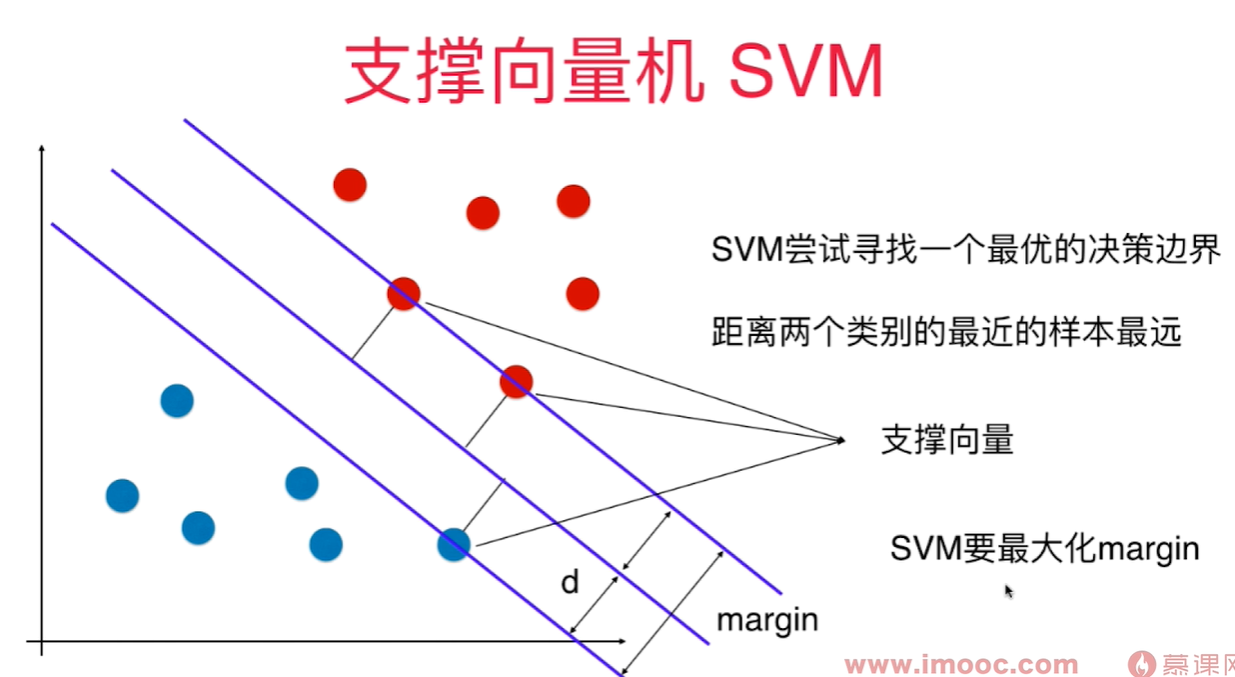
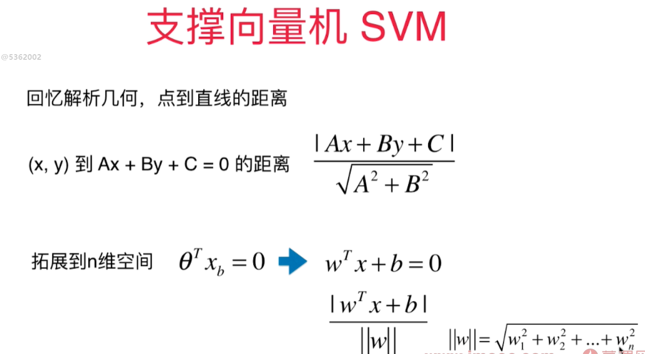
SVM - support vector machine 支撑向量机
不适定问题 - 决策边界不唯一
需要找到一条线,能很好的区分两种类别,同时临近直线的样本点离这条直线要尽可能远。
找到一个决策边界,不仅能对训练数据集进行很好的划分, 同时,泛化能力尽可能好!对泛化能力考量没有放在预处理阶段,而是放在算法内部。 - 统计学习中非常重要的方法。
margin 是和决策边界平行的两条直线间的距离,这两条直线分别穿过两类样本的临近点。
线性可分问题: 存在一个超平面,可以把两类样本分开 - Hard Margin SVM
真实环境中样本可能是线性不可分的,所以是一个Soft margin SVM 算法
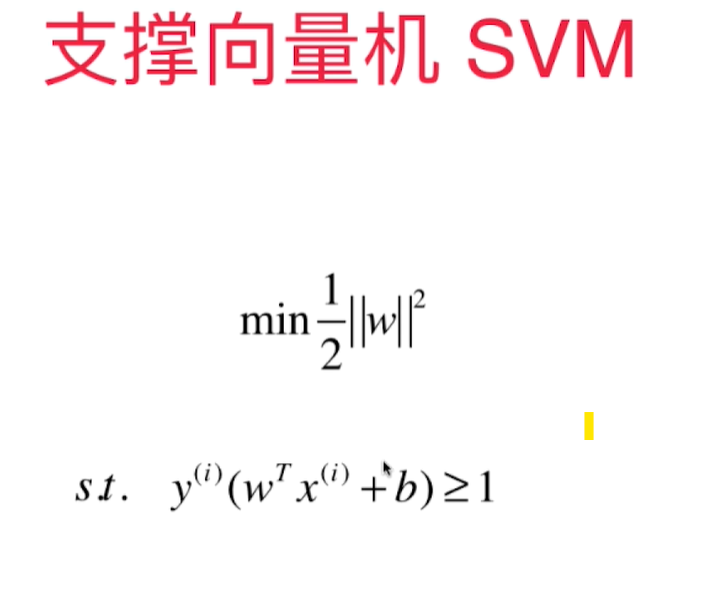
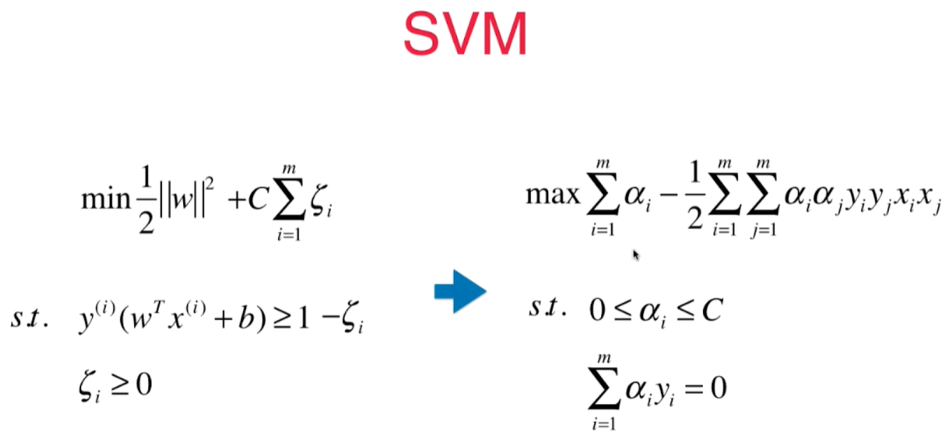
SVM 背后的最优化问题
所有的样本点到决策边界的距离都应该是 $ >= d$
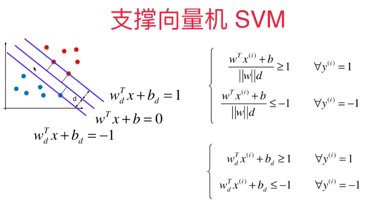
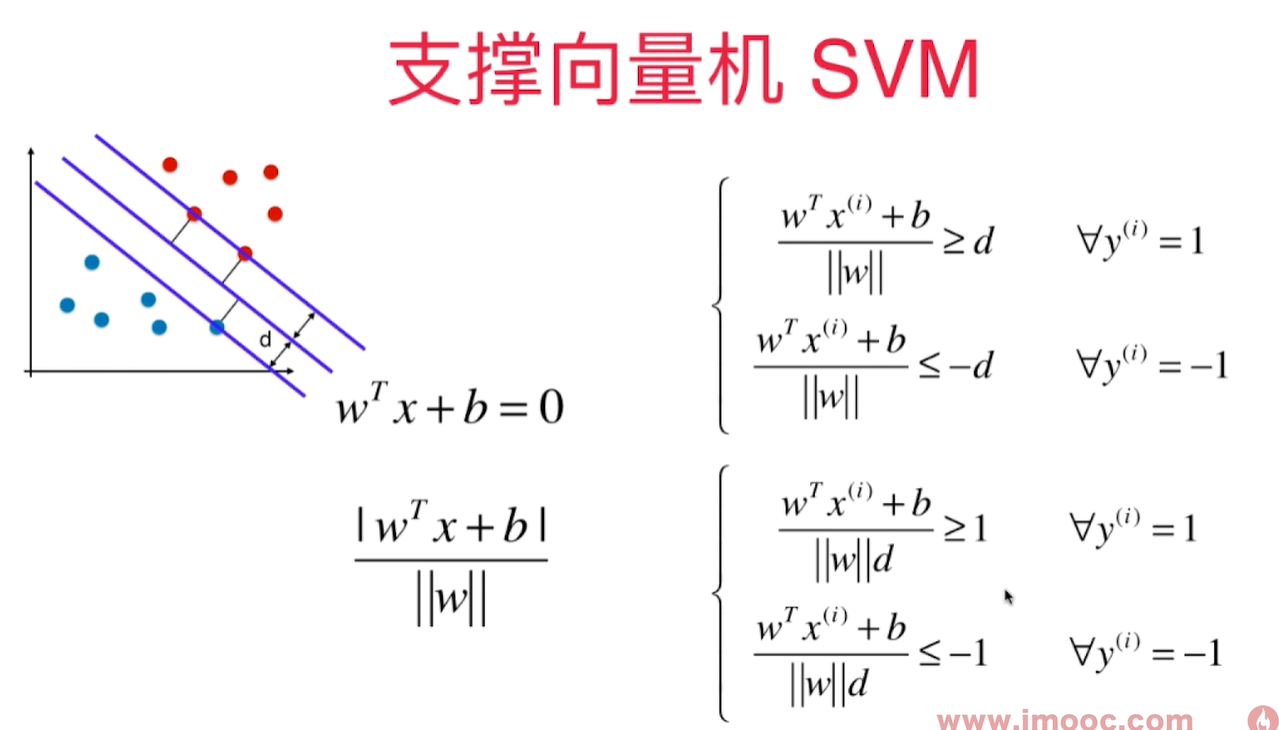
SVM的最优化问题:
Soft Margin SVM 和SVM 正则化
scikit-learn中的SVM
SVM中使用多项式特征和核函数
核函数 - 多项式核为例
SVM 求解一个有条件的最优化问题,在数学上需要变形成另一个数学问题:
在多项式 SVM中,$x_ix_j$ (向量点积)需要将两个向量添加上多项式项再进行运算, 核函数就是不需要先做多项式转换, 而通过一个函数(核函数)直接计算出多项式转换之后的点乘运算结果
$$K(x^{(i)}, x^{(j)}) = x^{'(i)}x^{'(j)}$$

kernel function - kernel trick(技巧)
变形通常是把一个低维样本变成高维数据,会花很多存储空间。 核函数可以避免这个过程,可以减少计算量,和存储空间, 降低计算复杂度。 - 不是SVM特有的技巧!
二次多项式核函数:
**$$K(x, y) = {(x\cdot y+1)}^2$$ **
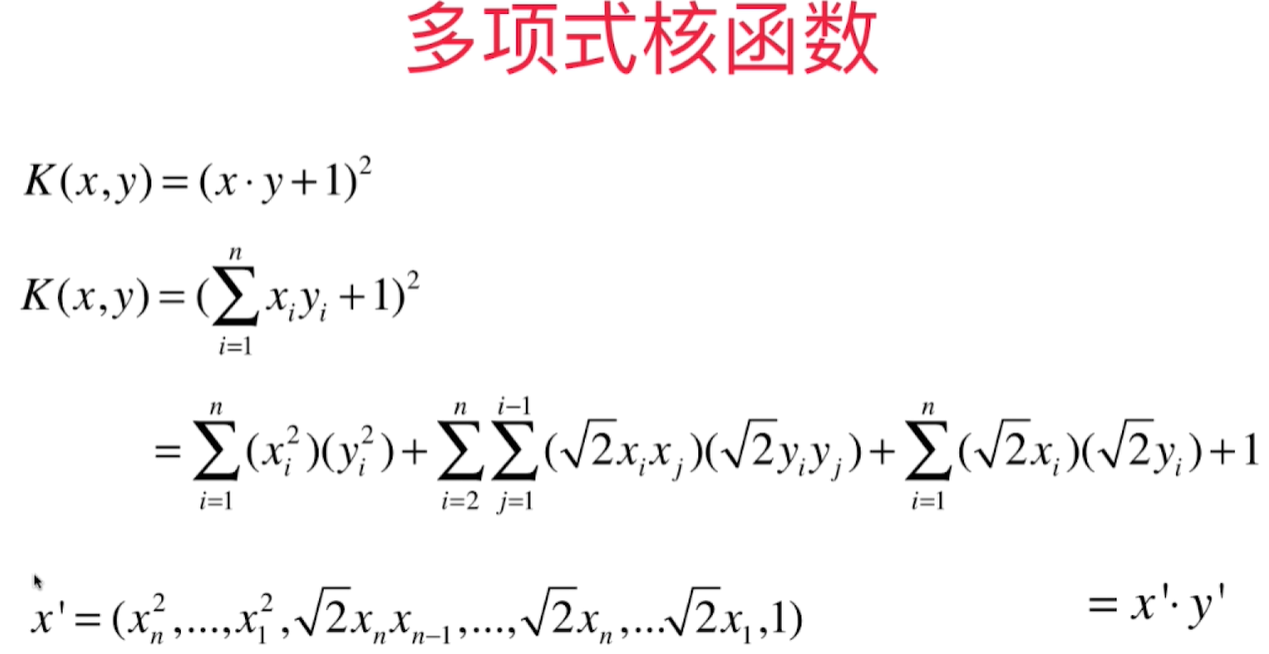
这个核函数就是在原来样本上添加了二次方的数据。有些参数前面有 $\sqrt 2$, 因为这只是一个系数,在求解出来的系数里除去这个系数即可,不影响功能。 通过核函数,不再需要将二次方数据得到然后做运算,而是通过原来的样本数据即可以运算得到添加二项式项之后的运算结果。
多项式核函数:
$$K(x, y) = {(x\cdot y+C)}^d$$ C和d(degree)是超参数
线性核函数
$$K(x, y) = {(x\cdot y)}$$
高斯核函数
$K(x, y)$ 表示x和y的点乘: $$K(x, y) = e^{-\gamma {\rVert x - y\rVert}^2}$$
Radio Basis Function Kernel(RBF核)
将原来的样本点映射成新的数据向量,再做点乘。- 将每一个样本点映射到一个无穷维的特征空间
多项式特征是依靠升维使得原本线性不可分的数据线性可分。
landmark $l_1, l_2$ 地标 假设有2个地标 $l_1, l_2$, 对于每一个x,将其映射为一个二维坐标如下:
$$ x \to (e^{-\gamma {\rVert x - l_1\rVert}^2}, e^{-\gamma {\rVert x - l_2\rVert}^2}) $$
因为在高斯核函数中,每一个样本点都是一个landmark,每个样本点都要对所有样本点做运算, 因此它是将m*n的数据映射成了m*m的数据。
高斯核函数计算开销大,初始样本维度很高,但是样本点不多,及m < n的情况下,则用RBF有优势。
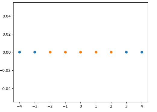
高斯核函数将1维数据映射到二维空间
一维数组,> -2, < 2的数为1, 其他为0, 在一维空间无法区分
import numpy as np
import matplotlib.pyplot as plt
x  = np.arange(-4, 5, 1)
y = np.array((x >= -2) & (x<=2), dtype = 'int')
plt.scatter(x[y==0], [0]*len(x[y==0]))
plt.scatter(x[y==1], [0]*len(x[y==1]))
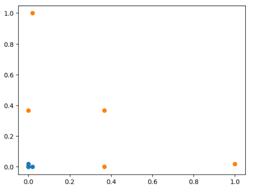
通过RBF转换为二维数组:
def gaussian(x, l):
    gamma = 1.0
    return np.exp(-gamma * (x - l)**2)

l1, l2 = -1, 1

X_new = np.empty((len(x), 2))
for i, data in enumerate(x):
    X_new[i, 0] = gaussian(data, l1)
    X_new[i, 1] = gaussian(data, l2)

plt.scatter(X_new[y==0, 0], X_new[y==0, 1])
plt.scatter(X_new[y==1, 0], X_new[y==1, 1])
Question, [0] 无法理解: 生成一个和第一个参数长度相等的值为0的数组
plt.scatter(x[y==0], [0]*len(x[y==0]))
plt.scatter(x[y==1], [0]*len(x[y==1]))
RBF核函数中的gamma
在高斯分布中, $\mu$ 代表高斯分布中的中心轴的位置; $\sigma$ 代表标准差,描述样本数据分布的情况!$\sigma$ 越小,分布曲线越窄,越大,分布曲线越缓,越宽. $$K(x, y) = e^{-\gamma {\rVert x - y\rVert}^2}$$
RBF里: gamma越大,高斯分布越窄; gamma越小,高斯分布越宽。
测试数据:
import numpy as np
import matplotlib.pyplot as plt
from sklearn import datasets
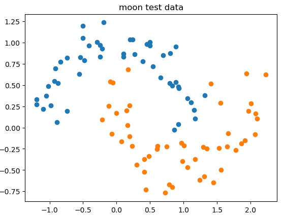
X, y = datasets.make_moons(noise = 0.15, random_state=666)
plt.scatter(X[y==0, 0], X[y==0, 1])
plt.scatter(X[y==1, 0], X[y==1, 1])
 gamma值为1时的决策边界:
from sklearn.preprocessing import StandardScaler
from sklearn.svm import SVC
from sklearn.pipeline import Pipeline
def RBFKernelSVC(gamma = 1.0):
    return Pipeline([
    ("std_scaler", StandardScaler()),
    ("svc", SVC(kernel="rbf", gamma = gamma))
    ])
svc = RBFKernelSVC()
svc.fit(X, y)
def plot_decision_boundary(model, axis):
    x0, x1 = np.meshgrid(
        np.linspace(axis[0], axis[1], int((axis[1] - axis[0])*100)).reshape(-1, 1),
        np.linspace(axis[2], axis[3], int((axis[3] - axis[2])*100)).reshape(-1, 1)
    )
    X_new = np.c_[x0.ravel(), x1.ravel()]

    y_predict = model.predict(X_new)
    zz = y_predict.reshape(x0.shape)

    from matplotlib.colors import ListedColormap
    custom_cmap = ListedColormap(['#EF9A9A', '#FFF59D', '#90CAF9'])
    plt.contourf(x0, x1, zz, cmap=custom_cmap)

plot_decision_boundary(svc, [-1.5, 2.5, -0.75, 1.25])
plt.scatter(X[y==0, 0], X[y==0, 1])
plt.scatter(X[y==1, 0], X[y==1, 1])
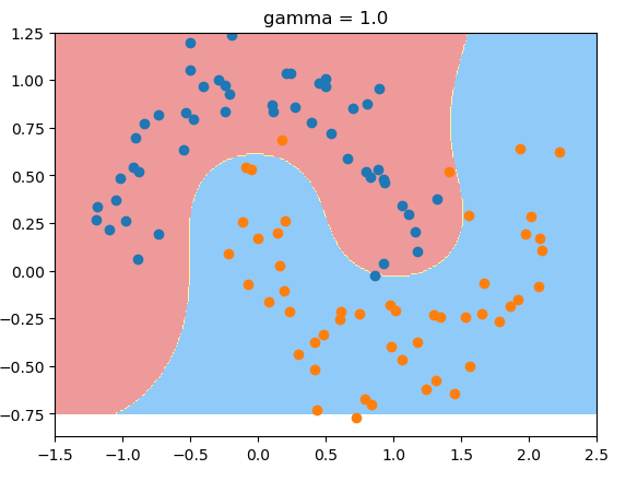
gamma值为100时,过拟合:
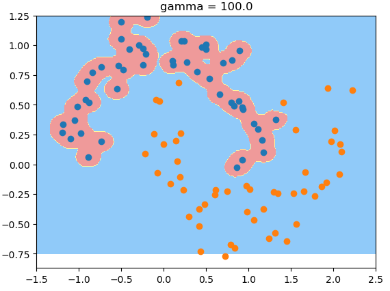
gamma值为0.1时,欠拟合:
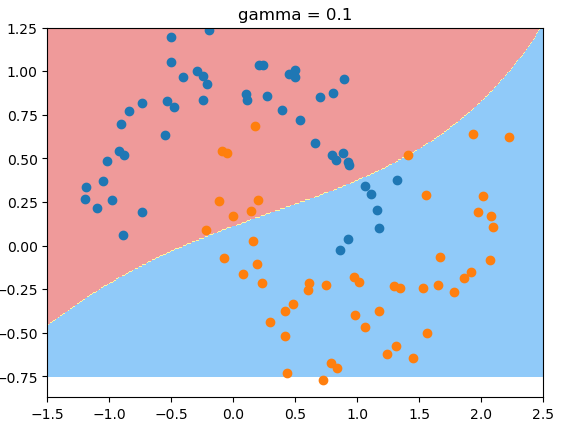
gamma值实际上在调整模型的复杂度,当gamma值越小,则模型复杂度越低(underfitting)。gamma越高 复杂度越高(overfitting).
使用SVM解决回归问题
决策树
是一颗数,有深度depth
- 非参数学习算法
- 可以解决分类问题
- 天然可以解决多分类问题
- 也可以解决回归问题(根据各个阈值沿着树最终会分到一个叶子节点,回归问题的预测值就是把分到某一类的样本点做一个平均值)
- 具有非常好的可解释性
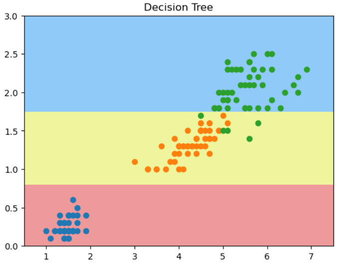
在某一个维度选择一个阈值
信息熵
信息熵在信息论中代表随机变量不确定的度量。- 系统中的不确定性的度量
- 熵越大,数据的不确定性越高
- 熵越小,数据的不确定性越低
热力学中引申出来: 熵越大,在一个热力系统中 ,那些粒子无规则运动就越剧烈;不确定性越高; 熵越小,粒子越倾向于静止,确定性越高!
$$H = - \sum_{i=1}^k p_i log(p_i) $$
$$H = -x log(x) - (1-x) log(1-x)$$
画出二分类的entropy曲线:
import numpy as np
import matplotlib.pyplot as plt
def entropy(p):
    return -p * np.log(p) - (1-p) * np.log(1-p)
x = np.linspace(0.01, 0.99, 100);
plt.plot(x, entropy(x))
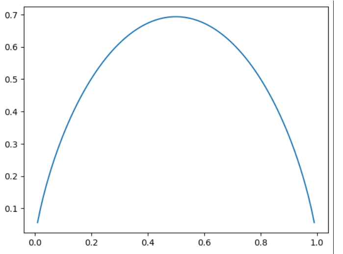 从图中可知,当两者概率都是0.5的时候,熵是最大的,最不确定的。
在决策树中,在每个节点上都是在一个维度上对数据做划分,划分的结果是使得系统整体的信息熵降低。 让系统变得更加确定。 最终,每个叶子上都是相同的数据集,这时候系统的熵为0。 - 通过搜索获得最好的划分(熵最低)
使用信息熵寻找最优划分
鸢尾花二维数据:
import numpy as np
import matplotlib.pyplot as plt
from sklearn import datasets
data = datasets.load_iris()
X = data.data[:, 2:]
y = data.target
from sklearn.tree import DecisionTreeClassifier
dtc_clf = DecisionTreeClassifier(max_depth = 2, criterion='entropy')
dtc_clf.fit(X, y)

def plot_decision_boundary(model, axis):
    x0, x1 = np.meshgrid(
        np.linspace(axis[0], axis[1], int((axis[1] - axis[0])*100)).reshape(-1, 1),
        np.linspace(axis[2], axis[3], int((axis[3] - axis[2])*100)).reshape(-1, 1)
    )
    X_new = np.c_[x0.ravel(), x1.ravel()]

    y_predict = model.predict(X_new)
    zz = y_predict.reshape(x0.shape)

    from matplotlib.colors import ListedColormap
    custom_cmap = ListedColormap(['#EF9A9A', '#EFF59D', '#90CAF9'])

    plt.contourf(x0, x1, zz, cmap=custom_cmap)

plot_decision_boundary(dtc_clf, [0.5, 7.5, 0, 3])
plt.scatter(X[y==0, 0], X[y==0, 1])
plt.scatter(X[y==1, 0], X[y==1, 1])
plt.scatter(X[y==2, 0], X[y==2, 1])
plt.title("Decision Tree")
和老师的结果有出入,第一个决策点不在x轴上,而在y轴上?
自己编写通过entropy来分类的决策树代码
from collections import Counter
def split(X, y, d, value):
    index_a = X[:, d] <= value
    index_b = X[:, d] > value
    return X[index_a], X[index_b], y[index_a], y[index_b]

def entropy(y):
    counter = Counter(y)
    res = 0.0
    for v in counter.values():
        p = v/len(y)
        res += -p * np.log(p)
    return res

def try_split(X, y):
    best_entropy = float('inf')
    best_d, best_v = -1, -1
    for d in range(X.shape[1]):
        sorted_index = np.argsort(X[:, d])
        for i in range(1, len(X)):
            if X[sorted_index[i-1], d] != X[sorted_index[i], d]:
                v = (X[sorted_index[i-1], d]+X[sorted_index[i],d])/2
                X_l, X_r, y_l, y_r = split(X, y, d, v)
                e = entropy(y_l) + entropy(y_r)
                if e < best_entropy:
                    best_entropy, best_d, best_v = e, d, v
    return best_entropy, best_d, best_v
求第一个决策点:
best_entropy, best_d, best_v =  try_split(X, y)
print("best_entropy = ", best_entropy)
print("best_d = ", best_d)
print("best_v = ", best_v)
结果:
best_entropy, best_d, best_v =  try_split(X, y)
print("best_entropy = ", best_entropy)
print("best_d = ", best_d)
print("best_v = ", best_v)
(0.6931471805599453, 0, 2.45)
求第二个决策点
X_l, X_r, y_l, y_r = split(X, y, 0, 2.45)
best_entropy2, best_d2, best_v2 = try_split(X_r, y_r)
print("best_entropy = ", best_entropy2)
print("best_d = ", best_d2)
print("best_v = ", best_v2)
X2_l, X2_r, y2_l, y2_r = split(X_r, y_r, 1, 1.75)
entropy(y2_l)
entropy(y2_r)
best_entropy =  0.4132278899361904
best_d =  1
best_v =  1.75

0.30849545083110386
0.10473243910508653
基尼系数
$$ G = 1 - \sum_{i=1}^k p_i^2 $$
$$G = 1 - x^2 - (1-x)^2 = -2x^2 + 2x$$
当x=1/2时,达到极值。
因为计算信息熵需要计算log,是一个非线性函数,计算比基尼系数稍慢。
sklearn中默认使用基尼系数做决策。
大多数时候二者没有特别的效果优劣。
信息熵对应的曲线本质上不是抛物线,基尼系数对应的曲线是一条抛物线。
CART 与决策树中的超参数
CART: Classification and Regression Tree
根据某一个维度d和某一个阈值v进行二分类。
SKlearn中的决策树用CART机制实现。其他可以用ID3, C4.5, C5.0来实现。
容易产生过拟合(和kNN一样), 所以必须剪枝,这样可以降低复杂度,解决过拟合。 max_depth = 2
不带参数时,会一直分类到gini系数为0, 所以会过拟合。
min_samples_split: 可以进一步拆分的最小样本数量 min_samples_leaf: 对于叶子节点最小可以有多少个样本
max_leaf_nodes:最多可以有多少个叶子节点
决策树解决回归问题
决策树可以解决分类问题,如果将分到某一个类的所有的样本的平均值作为被预测样本的值,则决策树可以解决回归问题。
决策树的局限性
局限性: 决策边界是横平竖直的,真实的决策边界可能是一条斜线,而决策树永远不可能产生这样的决策边界。 对于一个二分类清晰的样本,假如旋转一个角度,则会导致产生的决策边界是锯齿形的,而这个边界的远端肯定是不对的,因为它不是一条斜线。
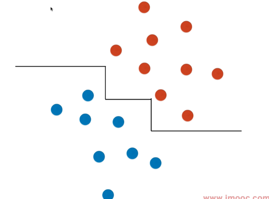
对个别数据点非常敏感。 - 非参数学习算法的共同特点 - 非常依赖于调参
看到书上说,sklearn中的决策树使用的算法是随机的,即对于每个决策树的节点都是随机选择 特征集进行评估,所以,得到的特征边界会不一样。 也证明了对数据点很敏感。
集成学习(ensemble learning)
同一个问题,不同算法会给出不同的结果。 把多个算法集中起来,都对同一个问题做计算,通过投票的方式,少数服从多数,得到最终的结果。
买东西找朋友推荐?综合多方面意见
病情确诊?- 专家会诊
Voting Classifier:
vc_clf_hard = VotingClassifier(estimators=[
 ('log_clf', LogisticRegression()),
 ('svm_clf', SVC()),
 ('dt_clf', DecisionTreeClassifier(random_state=666))
], voting = 'hard')
集成学习的方式提高了预测准确度。
Soft Voting Classifier
Hard Voting: 少数服从多数 Soft Voting: 基于权值的投票
民主暴政: 一人一票结果反而不好,最好是对不同的算法的结果应该要有权值的。 唱歌比赛的投票,那些老师权值高。 对于经济政策的推出,经济领域的专家的意见权值应该更高!
虽然只有2个模型的预测结果是A类,但是他们都非常确定结果是A类。 有3个模型将结果分成B类,但是每一个的预测概率并不高。
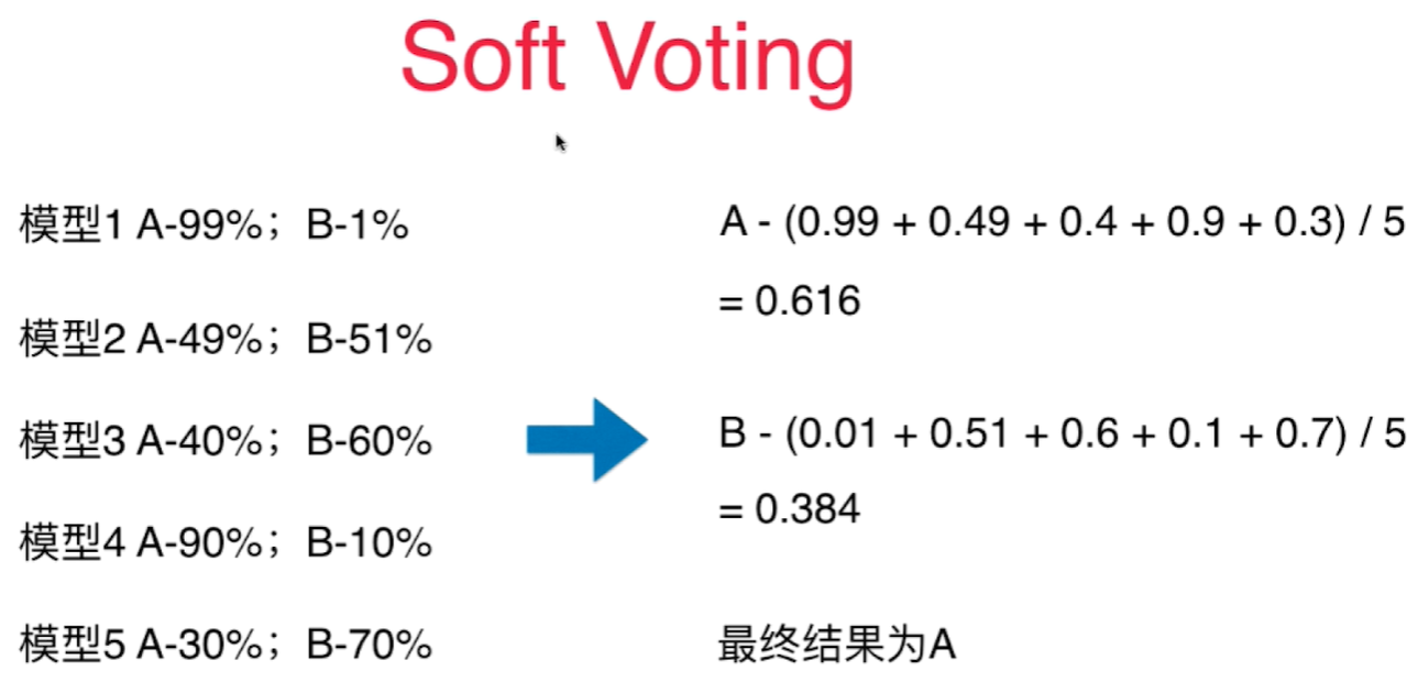
对分类结果的概率求和做平均,得到最终的概率,根据这个概率值来决定最终的分类结果。 - Soft Voting
- 要求集合的每一个模型都能估计概率
SVM算法目的是寻找最大的margin,没有考虑计算概率。但是SVC中有一个probability参数,默认是False,而设成True时会计算每个预测值的概率,但会牺牲性能。
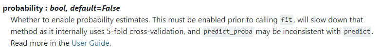
测试数据:
import numpy as np
from sklearn.model_selection import train_test_split
import matplotlib.pyplot as plt
from sklearn import datasets
X, y = datasets.make_moons(n_samples = 300, noise = 0.3, random_state=42)
X_train, X_test, y_train, y_test = train_test_split(X, y, random_state = 42)
plt.scatter(X[y==0, 0], X[y==0, 1])
plt.scatter(X[y==1, 0], X[y==1, 1])
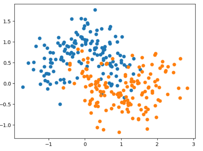
hard Voting:
from sklearn.ensemble import VotingClassifier
from sklearn.tree import DecisionTreeClassifier
from sklearn.svm import SVC
from sklearn.linear_model import LogisticRegression
vc_clf_hard = VotingClassifier(estimators=[
 ('log_clf', LogisticRegression()),
 ('svm_clf', SVC()),
 ('dt_clf', DecisionTreeClassifier(random_state=666))
], voting = 'hard')
vc_clf_hard.fit(X_train, y_train)
vc_clf_hard.score(X_test, y_test)
结果:
0.88
Soft Voting:
vc_clf = VotingClassifier(estimators=[
 ('log_clf', LogisticRegression()),
 ('svm_clf', SVC(probability=True)),
 ('dt_clf', DecisionTreeClassifier(random_state=666))
], voting = 'soft')
vc_clf.fit(X_train, y_train)
vc_clf.score(X_test, y_test)
结果:
0.9066666666666666
Bagging and Pasting
如何保证每个子模型创建的差异性: 每个子模型只看样本数据的一部分。
每个子模型的预测准确率低 - 并不需要太高的准确率。
如果每个子模型的预测准确率是60%, 500个子模型,总的准确率是: $$\sum_{i=251}^{500} C_{500}^i \cdot 0.6^i \cdot 0.4^{500-i} = 99.999% $$
在算法比赛中,集成学习的使用率是最高的。
每个子模型只看样本数据的一部分:
- 放回取样 - Bagging
- 不放回取样 - Pasting - 每个模型看到的样本是不重复的,不一样的
Bagging更常用, 如果不放回取样,则训练子模型数量太少。 - 统计学中叫 bootstrap Bagging没有特别依赖于随机,pasting中,分子样本会强烈影响集成学习所得的结果。
DecisionTreeClassifier 产生差异较大的模型,更加随机,集成学习要求子模型有区别,所以, 一般都用决策树做集成学习。
OOB(Out of Bag) 和关于Bagging的更多讨论
放回取样会导致一部分样本很可能没有取到。$37%$ - Out of bag
使用这些没有用过的样本做测试/验证就好了。 - 不需要再做训练/测试数据集分离了。 - 创建时加上bootstrap=True参数
oob_score_
%%time
bagging_clf2 = BaggingClassifier(DecisionTreeClassifier(), n_estimators=5000, max_samples=100, bootstrap=True) # bagging - 放回取样
bagging_clf.fit(X, y)
bagging_clf.oob_score_#读取验证的结果
结果:
CPU times: total: 781 ms
Wall time: 1.01 s
Bagging的思路极易做并行化处理,因为每一个子模型是独立的。- 创建时加上n_jobs=-1,充分利用多核处理器
%%time
bagging_clf = BaggingClassifier(DecisionTreeClassifier(), n_estimators=500, max_samples=100, bootstrap=True, oob_score = True, n_jobs=-1) # bagging - 放回取样
bagging_clf.fit(X, y)
结果:
CPU times: total: 297 ms
Wall time: 1.18 s
让每一个子模型产生差异化:
- 每个子模型使用一个小的样本集
- 针对特征进行随机采样 - Random Subspaces - 随机子空间
- 既针对样本,又针对特征进行随机采样 - Random Patches - 2个维度都是随机的,产生的图片就像一块有很多补丁的布

在特征空间进行随机采样的方式又叫 bootstrap_features。 max_features #每次随机采样的特征数量 bootstrap_features=True#激活特征空间随机采样
bagging_clf = BaggingClassifier(DecisionTreeClassifier(), n_estimators=500, max_samples=100, bootstrap=True, oob_score = True, n_jobs=-1, max_features=1, bootstrap_features=True) # bagging - 放回取样
bagging_clf.fit(X,
bagging_clf.oob_score_
结果:
0.8466666666666667# 因为总共只有2个特征,效果不明显
用决策树实现的BaggingClassifier就是随机森林,因为每一个子模型都是一个决策树。
测试代码:
import numpy as np
from sklearn.model_selection import train_test_split
import matplotlib.pyplot as plt
from sklearn import datasets
X, y = datasets.make_moons(n_samples = 300, noise = 0.3, random_state=42)
X_train, X_test, y_train, y_test = train_test_split(X, y, random_state = 42)
plt.scatter(X[y==0, 0], X[y==0, 1])
plt.scatter(X[y==1, 0], X[y==1, 1])
| BaggingClassifier() | Parameters |
|---|---|
| 每个子模型只看样本数据的一部分 | bootstrap=True, max_samples=?, n_estimators=? |
| 每个子模型只看样本特征集的一部分 | bootstrap_features=True, max_features=? |
| Random Patches |
随机森林和Extra-Trees
随机森林中,决策树在节点划分上,在随机的特征子集上寻找最优划分特征。
from sklearn.ensemble import RandomForestClassifier
rfc = RandomForestClassifier(n_estimators=500, random_state=666, oob_score=True, n_jobs=-1)#有500个子决策树模型
rfc.fit(X, y)
rfc.oob_score_

rfc = RandomForestClassifier(n_estimators=500, max_leaf_nodes=16,  random_state=666, oob_score=True, n_jobs=-1)#有500个子决策树模型
Extremely random trees: Extra-Trees - 极其随机森林
决策树在节点划分上,使用随机的特征和随机的阀值.
提供了额外的随机性, 抑制了过拟合,不会被一些特别的点带偏(因为每一棵树都是极其随机的),但是增加了bias(偏差),减少了方差。
from sklearn.ensemble import ExtraTreesClassifier
etc = ExtraTreesClassifier(n_estimators=500, random_state=666, oob_score=True, bootstrap=True)
etc.fit(X, y)
etc.oob_score_
同样也有对应的Regressor:
from sklearn.ensemble import BaggingRegressor
from sklearn.ensemble import RandomForesetRegressor
from sklearn.ensemble import ExtraTreesRegressor
Ada Boosting 和Gradient Boosting
Boosting 类的算法,有分类器,也有回归器
from sklearn.ensemble import AdaBoostingRegressor
from sklearn.ensemble import GradientBoostingRegressor
集成多个模型,每个模型都在尝试增强(Boosting)整体的效果。
初始时,所有的样本点权重是一样的,在第二次训练时,增加和第一次拟合出来的曲线距离较远的点的权重,再拟合,第三次再对第二次拟合出来的曲线相距较远的点提高权重再拟合。每次拟合的算法可能不一样。
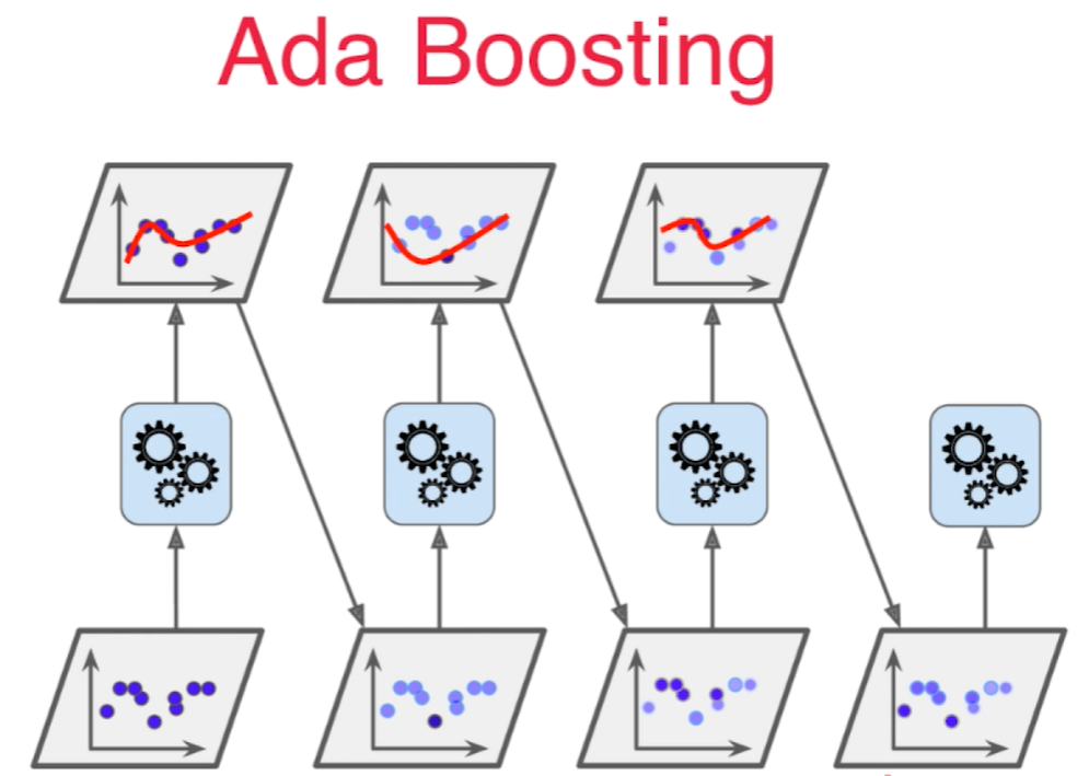
from sklearn.tree import DecisionTreeClassifier
from sklearn.ensemble import AdaBoostClassifier
ada_clf = AdaBoostClassifier(DecisionTreeClassifier(max_depth=2), n_estimators=500)
ada_clf.fit(X_train, y_train)
Gradient Boosting
对整体数据集用模型m1训练, 产生错误e1, 再用e1训练第二个模型m2, 产生错误e2,针对e2训练第三个模型m3,产生错误e3, ... 最终预测结果是: m1+m2+m3+...
每个模型都是对前一个模型所犯错误的补偿。
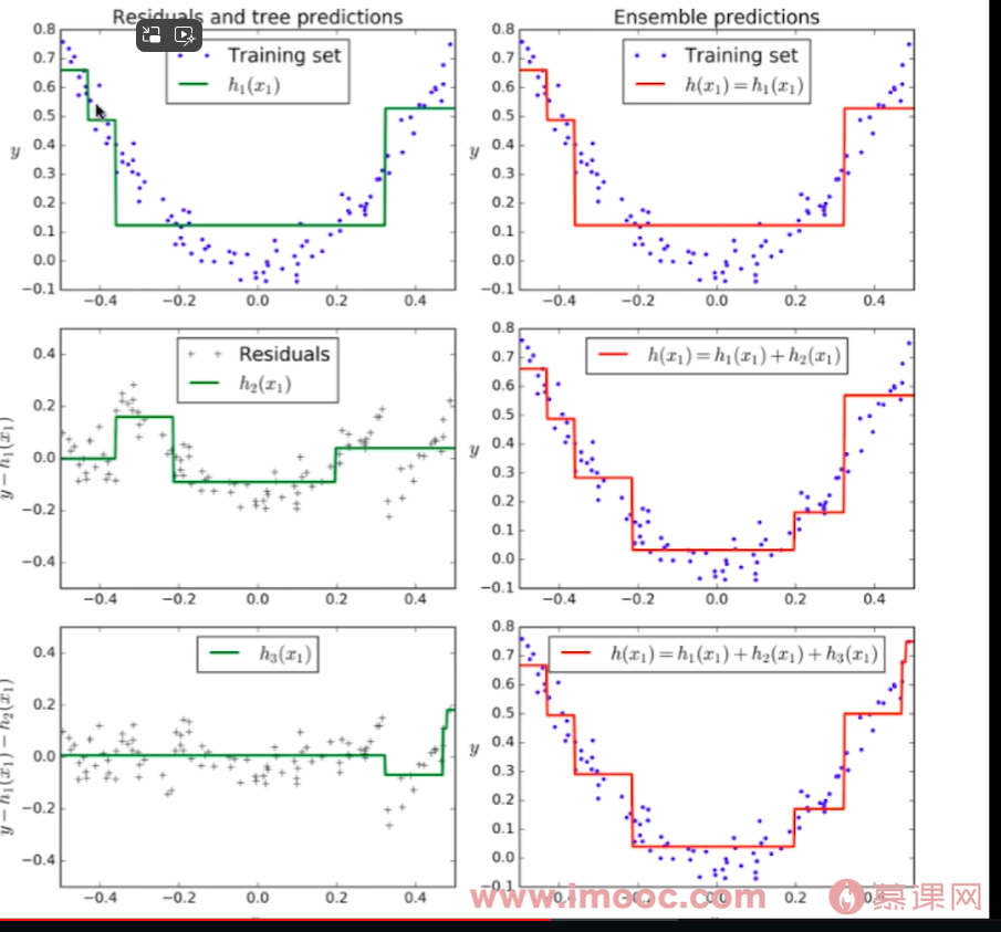
这种方法是基于决策树作为base estimator的,所以不像Ada Boosting,不需要设置base estimator。
from sklearn.ensemble import GradientBoostingClassifier
gb_clf = GradientBoostingClassifier(max_depth=2, n_estimators=30)
gb_clf.fit(X_train, y_train)
gb_clf.score(X_test, y_test)
Stacking
先用三个模型得出预测结果,再用一个模型基于预测的结果得出最终的结果。
把训练集分成2分,第一份用于训练前3个模型,第二份用于训练第四个模型。
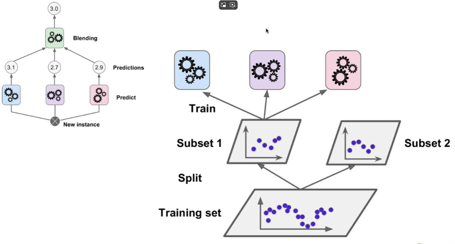
stacking模型的结构非常像神经网络
下面这个例子需要把数据分成3分,第一份训练第一层的3个模型,第二份训练第二层的3个模型,第三份训练第三层的模型,所以对于stacking来说,把模型分几层也是一个超参数。
