逻辑回归中使用正则化
多项式回归中引入L2 或 L1正则项:
$$J(\theta) + \alpha L_2 $$
$$J(\theta) + \alpha L_1 $$
引入一个新的正则化超参数: $C$
$$C\cdot J(\theta) + L1$$
$$C\cdot J(\theta) + L2$$
C越大(1000, 10000),则 $J(\theta)$ 的影响力越小. C越小,比如0.1, 0.01, 则L1/L2正则项更加重要, 因为L1/L2是$\theta$项, 也即 $\theta$ 项尽可能小。
正则项L1, L2, 正则项 $C$ 可以看成是 $L1$, $L2$ 前面的 $\alpha$ 的倒数。 在逻辑回归和SVM算法中,sklearn中的正则化更偏好用 $C$, 而不是用$\alpha$ .这样可以保证必须做正则化. 也提醒我们对于一些逻辑复杂的算法,都应该加上正则化。
sklearn中的LogisticRegression自带了正则化功能,有多个超参数可以配置:
- penalty, 'l2' in default
- C, 1.0 in default
- solver, lbfgs in default
- ......
决策边界为抛物线的测试代码:
import numpy as np
import matplotlib.pyplot as plt
np.random.seed(666)
X = np.random.normal(0, 1, size=(200, 2))# 有200个样本,每个样本2个特征
y = np.array(X[:, 0]**2 + X[:, 1] < 1.5, dtype='int')
for _ in range(20): # 加入20个噪音
    y[np.random.randint(200)] = 1
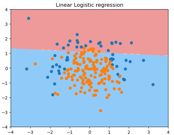
用线性逻辑回归拟合一个决策边界为抛物线的样本的结果:
from sklearn.model_selection import train_test_split
X_train, X_test, y_train, y_test = train_test_split(X, y, random_state=666)
from sklearn.linear_model import LogisticRegression
log_reg = LogisticRegression()
log_reg.fit(X_train, y_train)
plot_decision_boundary(log_reg, axis=[-4, 4, -4, 4])
plt.scatter(X[y==0, 0], X[y==0, 1])
plt.scatter(X[y==1, 0], X[y==1, 1])
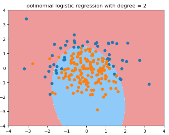
用度为2的多项式逻辑回归拟合的结果:
from sklearn.pipeline import Pipeline
from sklearn.preprocessing import PolynomialFeatures
from sklearn.preprocessing import StandardScaler
def PolynomialLogisticRegression(degree):
    return Pipeline([
        ('poly', PolynomialFeatures(degree = degree)),
        ('std_scaler', StandardScaler()),
        ('log_reg', LogisticRegression())
    ])
poly_log_reg = PolynomialLogisticRegression(degree=2)
poly_log_reg.fit(X_train, y_train)
plot_decision_boundary(poly_log_reg, axis=[-4, 4, -4, 4])
plt.scatter(X[y==0, 0], X[y==0, 1])
plt.scatter(X[y==1, 0], X[y==1, 1])
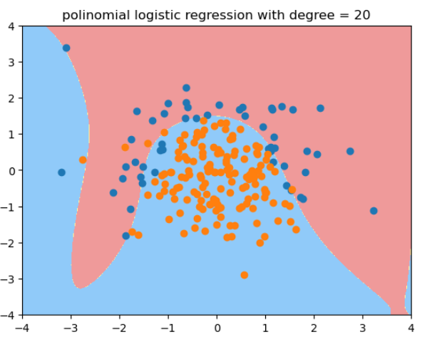
用度为20的多项式逻辑回归拟合的结果: -
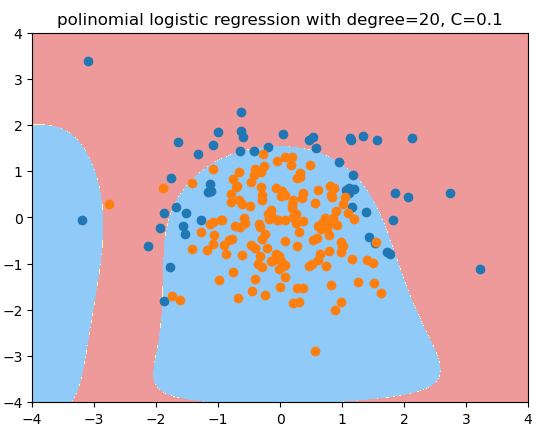
用度为20, C=0.1的多项式逻辑回归拟合的结果, 更倾向于degree=2的情况:
def PolynomialLogisticRegression(degree, C, penalty = 'l2', solver='liblinear'):
    return Pipeline([
        ('poly', PolynomialFeatures(degree = degree)),
        ('std_scaler', StandardScaler()),
        ('log_reg', LogisticRegression(C = C, penalty = penalty, solver=solver))
    ])
poly_log_regc = PolynomialLogisticRegression(degree=20, C=0.1, solver='liblinear')# 正则化权重大,分类损失函数权重小,
poly_log_regc.fit(X_train, y_train)
poly_log_regc.score(X_train, y_train)
poly_log_regc.score(X_test, y_test)
plot_decision_boundary(poly_log_regc, axis=[-4, 4, -4, 4])
plt.scatter(X[y==0, 0], X[y==0, 1])
plt.scatter(X[y==1, 0], X[y==1, 1])
plt.title("polinomial logistic regression with degree=20, C=0.1")
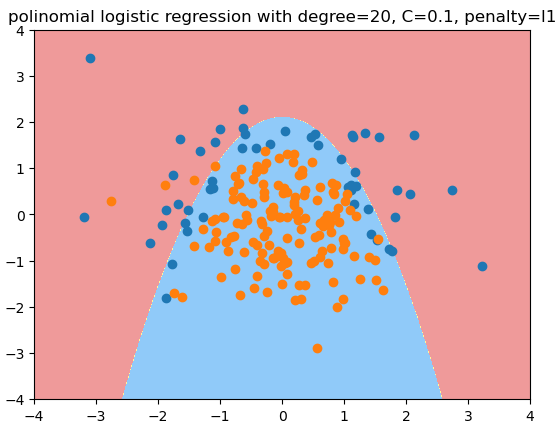
用度为20, C=0.1, penalty='l1'的多项式逻辑回归拟合的结果 - L1正则项可以减少很多多项式项,使其系数为0,逼近期望的结果 - 原始数据的形状
def PolynomialLogisticRegression(degree, C, penalty = 'l2', solver='liblinear'):
    return Pipeline([
        ('poly', PolynomialFeatures(degree = degree)),
        ('std_scaler', StandardScaler()),
        ('log_reg', LogisticRegression(C = C, penalty = penalty, solver=solver))
    ])
poly_log_regc = PolynomialLogisticRegression(degree=20, C=0.1, penalty = 'l1', solver='liblinear')# 正则化权重大,分类损失函数权重小,
poly_log_regc.fit(X_train, y_train)
poly_log_regc.score(X_train, y_train)
poly_log_regc.score(X_test, y_test)
plot_decision_boundary(poly_log_regc, axis=[-4, 4, -4, 4])
plt.scatter(X[y==0, 0], X[y==0, 1])
plt.scatter(X[y==1, 0], X[y==1, 1])
plt.title("polinomial logistic regression with degree=20, C=0.1, penalty=l1")
真实环境中,我们不知道哪个degree/C/penalty是最佳的超参数,只能通过网格搜索来获得。